After struggling through an accounting course in college, I decided Excel spreadsheets weren't for me. I would leave numbers and functions to the financial whizzes of the world. But as it turns out, spreadsheets aren't limited to just tracking profits and losses. You can use them to collect form submissions, manage projects, and organize your to-do list—among plenty of other tasks.
But before you can take advantage of all the data-crunching features Excel has to offer, you need to get the hang of the basics, like how to add data and how to use formulas. Here's everything you need to know about how to use Excel.
What is Microsoft Excel?
Microsoft Excel is a popular spreadsheet app used to organize, format, and calculate data.
If you have a paid Microsoft 365 subscription, you can use the desktop app. But anyone can use Excel online for free—it looks a lot like the desktop version with a few key differences.
What is Excel used for?
Excel is often used by accounting teams to store, visualize, and analyze data—especially larger data sets. But anyone in any field can use Excel to manage data. Here are a handful of ways you can use Excel:
Manage financial budgets and track expenses
Is Microsoft Excel the same as Google Sheets?
If you're familiar with Google Sheets, you'll notice a lot of overlapping features with Excel. You can read all about them in our Google Sheets vs. Microsoft Excel comparison, but here are the main takeaways:
Excel is the better tool for dealing with big data. Google Sheets has a limit of 10 million cells, but that pales in comparison to Excel's 17 billion cells per spreadsheet.
Excel has more powerful formulas and data analysis features, including built-in statistical analysis tools and extensive data visualization options. Google Sheets offers the "lite" version of most of those features, but it's nowhere near as in-depth.
Looking for an Excel alternative? Check out our list of the best spreadsheet software.
Microsoft Excel basic terms
Before we dive in, let's cover some spreadsheet terminology you'll need to know when using Microsoft Excel:
Cell: a single data point or element in a spreadsheet.
Column: a vertical set of cells.
Row: a horizontal set of cells.
Range: a set of one or more cells extending across a row, column, or both.
Function: a predefined formula built into the app used to manipulate data and calculate cell, row, column, or range values. For example, you can use the function
=SUMto calculate the total value of a given cell range.Formula: any equation designed by an Excel user to perform calculations, return information, and manipulate the contents of other cells. For example,
=A3+A10(this calculates the sum of values in cellsA3andA10). Note: You can combine functions and formulas.Worksheet (or spreadsheet): a single page of an Excel workbook.
Workbook: an Excel file containing one or more worksheets.
How to create an Excel spreadsheet
By default, when you create a new workbook in Excel, it'll open with a blank spreadsheet. There are three ways to create a workbook in Microsoft Excel online. To get started, log in to Microsoft 365.
Option 1: In the sidebar menu, click Create. In the Create dashboard, click Workbook.

Option 2: In the sidebar menu, click Excel. In the Create new section of your Excel dashboard, click Blank workbook.

Option 3: If you have a workbook open and want to create a new one, click File. From the Home side panel that appears, click New.

Using the desktop app? On the Home screen, click Blank Workbook.

The options listed above will open a workbook with a blank worksheet. But if you want to create a workbook to, say, track your tasks or create a budget, Excel offers prebuilt design templates to jumpstart the process. Or, you can work from your own spreadsheet template.
To add a spreadsheet to a workbook, click the New sheet icon, which looks like a plus sign (+), next to your existing sheet tab.

How to save an Excel file
If you're using Excel online, Excel automatically saves your work as you go. But if you want to save your workbook as a new file, here's how to manually save an Excel file.
Click File.
Click Save As, and then select Save a Copy. If you're using the desktop app, you have to click only Save As.
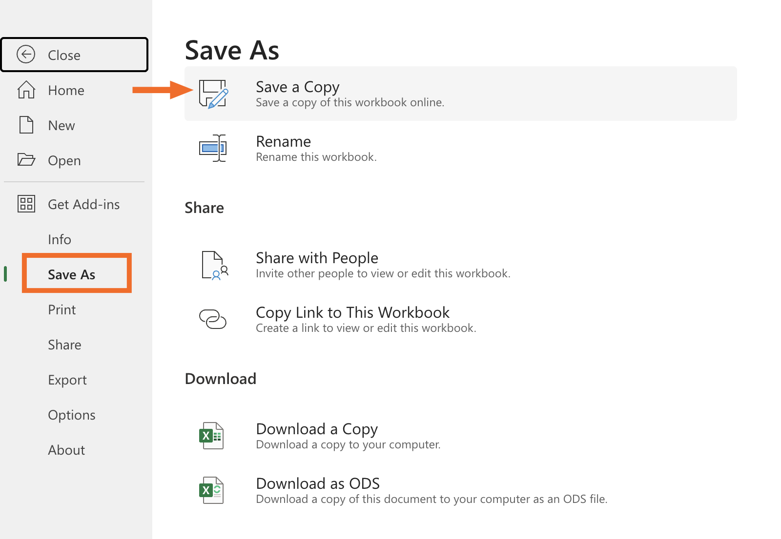
In the popup that appears, rename your file and choose where you want to store it. If you're using Excel online, you'll be able to store it only in OneDrive as an .xlsx file. If you're using the desktop app, you'll have the option to save it in OneDrive or to your computer in a few different formats—for example, .xls, .xlsx, and .csv.
Click Create a Copy (online) or Save (desktop app).


How to save an Excel file as a PDF
The steps to save an Excel file as a PDF differ depending on which version of the app you're using—online or desktop.
How to save an Excel file as a PDF using Excel online
Click File.
Click Export, and then select Download as PDF.

That's it. A PDF copy of your workbook will save to your computer.
How to save an Excel file as a PDF using the desktop app
Click File, and then select Save As.
Rename your file.
Click the dropdown next to File Format, and select PDF.
By default, Excel will save the entire workbook. But if you want to save only a specific sheet or selection of your workbook, you can change this.
Click Save.

How to add data to your spreadsheet
In a spreadsheet, data gets added to individual cells. To make it easier to filter or manipulate data later on, each cell should contain only one value. For example, 100 or Cincinnati.
Select the cell you want to add data to, and then type in the data. If you don't want to type in everything manually, you can also add data to your worksheet en masse using a few different methods:
Copy and paste a list of text or numbers into your spreadsheet.
Copy and paste an HTML table from a website.
Import an existing spreadsheet in
.csv,.xls,.xlsx, and other formats. (Better yet, you can link your spreadsheets to keep the data consistent.)Drag the fill handle across any row or down any column to automatically populate the highlighted cells with data.
How to use the fill handle in Excel
The fill handle in Excel offers a convenient way to populate data or copy formulas and data in adjacent cells. Hover your cursor over the bottom-right corner of any cell or cell range, and it'll automatically turn into the fill handle, which looks like a plus sign (+).

By dragging the fill handle across or down a range of cells, you can perform a number of tasks:
Copy a cell's data to neighboring cells (including formatting).
Copy a cell's formula to neighboring cells.
Create an ordered list of data.
How to use the fill handle to copy a cell's data to neighboring cells
Highlight the cell or range of cells containing the data you want to copy. Drag the fill handle across the row or down the column.
If you select only one cell, the value of the selected cell will appear in every cell that you drag the handle over.

If you select a series of neighboring cells, Excel will repeat the pattern across or down the cells that you drag the handle over. In the example below, I've selected three neighboring cells, each containing a unique value: Denver, Tucson, and Cleveland. When I drag the fill handle, the pattern repeats across the row so that it's Denver, Tucson, Cleveland, Denver, Tucson, Cleveland, and so on.

How to use the fill handle to copy a cell's formula to neighboring cells
Highlight the cell containing the formula you want to copy. Drag the fill handle across the row or down the column. The formula will automatically (or dynamically) update to match the relevant row.
In the example below, I've entered the formula =SUM(B3:F3) in cell G3, which tells Excel to calculate the total value of cells B3 to F3 (or columns B to F in only row three).
Note: cell ranges in Excel are indicated using a colon (:), as shown in the example below. A series of specific cells, however, are separated by commas (,). For example, =SUM(B3,D3,F3) would calculate the total for only cells B3, D3, and F3.

When I drag the fill handle down the Total column (column G), Excel assumes I want to calculate the values of columns B to F for each row, so it dynamically updates the formula to =SUM(B4:F4), =SUM(B5:F5), and so on.

Note: If you run into issues using the fill handle to copy formulas into adjacent cells, you may need to check the cell references (any cells referenced in that cell's formula) of the first cell.
How to use the fill handle to create an ordered list
Let's say you've added the following data to three neighboring cells: Employee 1, Employee 2, and Employee 3. To continue the ordered list, highlight the three cells and drag the fill handle across the row or down the column. Excel will continue the ordered list.

There are a few caveats worth mentioning, though.
In some cases, you may need to highlight at least two cells containing the sequence you want Excel to continue. If you select only
Employee 1and drag the handle across, Excel may repeatEmployee 1in the neighboring cells.Unlike copying text values to neighboring cells, Excel will only continue sequences for number values—not repeat them. For example, if I wanted to repeat the sequential pattern
Employee 1,Employee 2, andEmployee 3across the row, Excel wouldn't be able to. It would just keep counting up. I would have to manually copy and paste the values across instead. To make things confusing, if I highlighted cells containing an arbitrary set of numbers, like1,17, and20, Excel would repeat this pattern since there's no logical sequence to continue.
How to format data in Excel
If you copied data from another source or manually entered it yourself, there's a good chance you'll want to edit and format it to make your spreadsheet easier to digest.
How to navigate the Excel ribbon
The ribbon—the row of tabs and tools at the top of your spreadsheet—allows you to quickly access common editing tools. Microsoft does a nice job of grouping closely related tools together within their respective tabs, making it easier to find what you need.
If you can't find a tool, or you want to check if a tool exists, the quickest way to access it is by using the Search bar. In Excel online, click the Search icon, which looks like a magnifying glass above the ribbon. In the desktop app, you can do the same thing or click Tell me at the top of the ribbon.

Want to hide the ribbon? In Excel online, click Ribbon Display Options, which looks like a down caret (⋁) in the bottom-right corner of the ribbon. Then click Automatically Hide.

Your ribbon will automatically disappear. To make it temporarily reappear, hover your cursor above your worksheet.
To hide the Excel ribbon in the desktop app, use the keyboard shortcut: Command+Option+R on a Mac or Ctrl+F1 on Windows. Press the shortcut again to make your ribbon reappear.
Now, back to using the tools in the ribbon.
Hover over any icon to discover its function. Or click on the down caret (⋁) beside an icon, if applicable, to expand that tool's options. Tools like Borders, Fill Color, and Align work similarly to what you'd expect from another word processor, like Microsoft Word.
The best way to show you how to use some of the most common Excel editing tools is to work through an example. Let's edit this simple student roster with test grades.

How to format text and data in Excel
The text and data formatting tools are in the Home tab of your ribbon. To start, let's make the headers in the top two rows stand out.
Click the cells you want to format. To apply the same formatting to neighboring cells, select the first cell and drag your cursor across or down the cell range. To apply the same formatting to cells that aren't connected, select one cell, press and hold
commandon a Mac orCtrlon Windows, and then select the other cells. Note: Your cell selection will remain selected unless you click on a different cell, which is convenient if you want to edit multiple formatting options.From the ribbon, click the down caret (
⋁) beside the Font Size and select 12. Or you can enter12in the font size field.Click the Bold icon, which looks like the letter
B.Click the down caret (
⋁) beside the Fill Color icon, which looks like a paint can, and select a theme color. I'm using a light shade of green.Click the Align icon, which looks like a stack of horizontal lines. In the Text Alignment section, click Center.
This grade sheet is already a little easier to scan through. But there are a few more edits to make.

How to merge cells in Excel
The header Tests applies to cells C2 to G2, but right now, it looks like it only applies to cell C2 (Unit 1). To make this clearer, let's merge cells C1 to G1.
Select cells C1 to G1.
From the ribbon, click the Merge icon, which looks like a horizontal line with arrowheads on both ends.
The five individual cells have now merged into one cell. And because we previously applied center alignment to all the headers, Tests automatically centers itself within the merged cells.

How to add leading zeros in Excel
The student ID numbers in column B should start with 000 (leading zeros). By default, if you enter a number that starts with zeros in Excel, like 0001, Excel will automatically ignore the leading zeros and display only 1 (or a non-zero digit). Here's how to force Excel to show leading zeros.
Select cells B3 to B9.
Click the down caret (
⋁) next to Number Format, and select Text.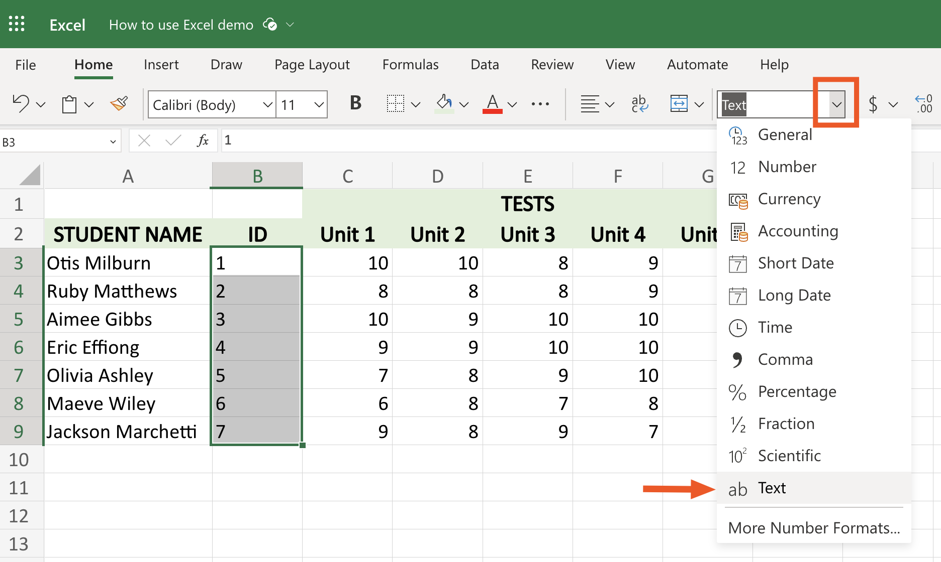
Enter
0001in cell B3.In this example, the student IDs are assigned in sequential order. To quickly populate their ID numbers, drag the fill handle from cell B3 down to cell B9.

Note: If your spreadsheet includes numbers formatted as text values, Excel can't calculate these values if they're referenced in a formula or function.
How to create a table in Excel
When you're staring at a large data set, it's easy for all those numbers and letters to become a blur. One way to make your spreadsheet less of an eyesore: format it as a table. It'll fill each row with an alternating color scheme, making it easier to differentiate one row of data from the next.
Highlight the data you want to include in your table.
In the Home ribbon, click the Format As Table icon.
Choose the color theme you want to use for your table.
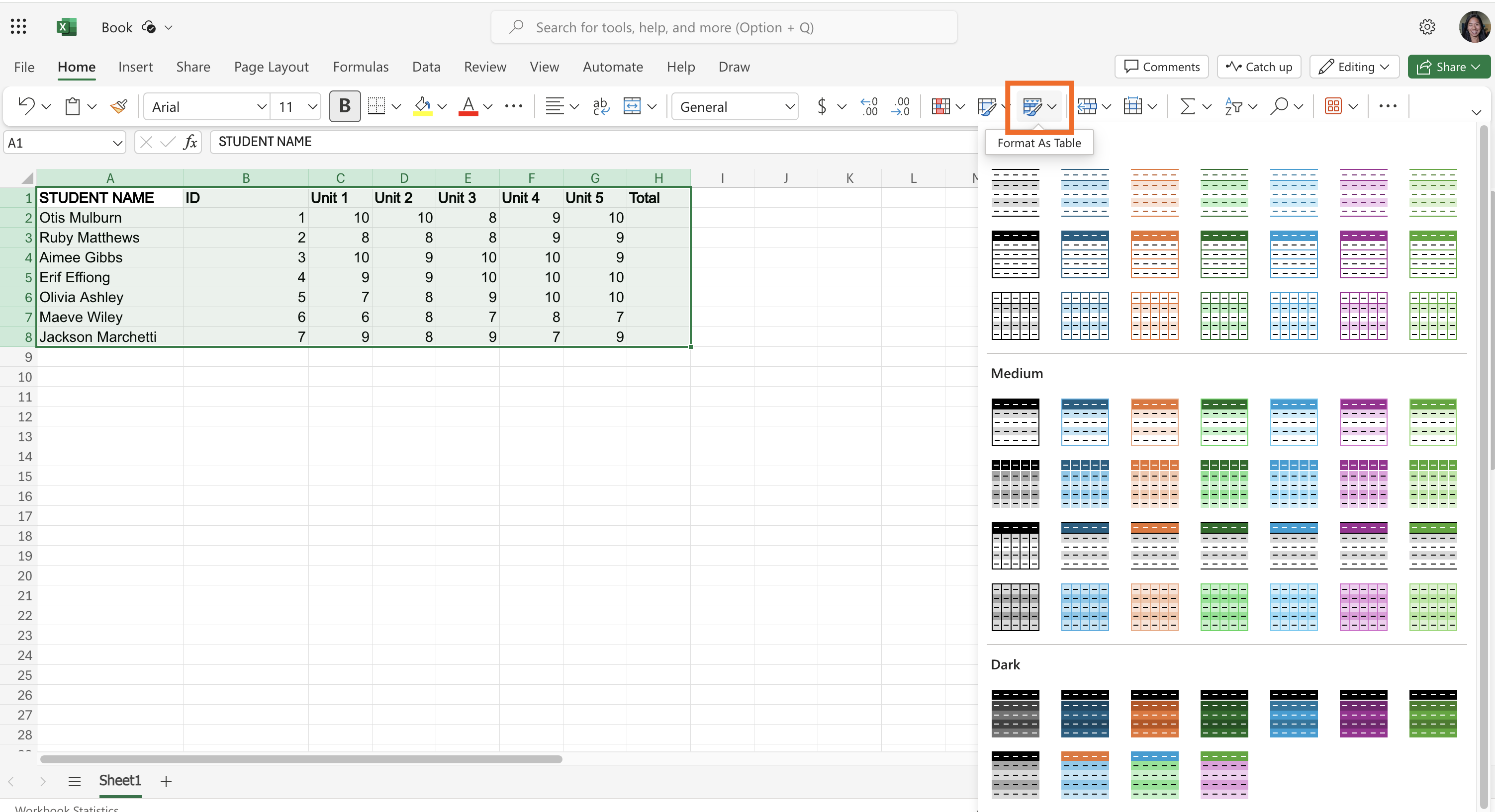
In the popup that appears, confirm the data range. Excel will also automatically detect if your data has headers, but if not, you can manually indicate this by checking the box next to My table has headers.
Click OK.


There you go: a beautifully formatted table in just a few clicks.

How to sort and filter in Excel
When you formatted your data as a table, Excel automatically added the ability to sort and filter your data. Here's how to use each feature.
How to sort data in Excel
Excel allows you to sort your data alphabetically (A to Z or Z to A) and from smallest to largest (or vice versa). It automatically knows which option to give you depending on the type of data contained in each column. For example, if it's filled with text values, it'll give you the option to sort alphabetically.
Click the down caret (
⋁) next to the header of the column you want to sort.Select how you want to sort your data.
In the example below, I've sorted student names reverse alphabetically.

How to filter data in Excel
There are countless ways you can filter data in Excel so I'll show you, generally, how to set your filters.
Click the down caret (
⋁) next to the column header with the data you want to filter.Click Text Filters or Number Filters (the option changes depending on the type of values contained in that column's cells).
Select a way to filter your data.
Depending on the filter you chose in the previous step, you might be prompted to enter the value you want Excel to sort the data by. For example, if you choose Equals, you'll be prompted to enter the exact value you want Excel to filter for.

How to edit rows and columns in Excel
How to insert rows and columns
Let's say you gave your students another test: unit 6. Now you need to add another column to capture their unit 6 test grades. This column should go between Unit 5 and Total in columns G and H.
Click H (this will highlight the entire column).
Right-click the column.
Select Insert Columns.

By default, Excel will insert a column to the left of whichever column was selected.

If you want to, say, insert three columns at once, select three adjacent columns, and repeat the steps above. Remember: Excel will insert these columns to the left of your selection.
To insert a row, select a row or multiple row numbers, and follow the same steps from above.
How to delete rows and columns
Select the column or row you want to delete.
Right-click your selection.
Click Delete Rows.
This will permanently delete your column or row. To quickly undo this action, use your keyboard shortcut: command+Z on a Mac or Ctrl+Z on Windows.
How to hide rows and columns
If specific rows or columns of data are cluttering your view, you can hide them.
Click the column letter or row number that you want to hide. You can also click multiple columns or rows to hide them at the same time.
Right-click the selection.
Click Hide Columns or Hide Rows.
In the example below, I've hidden the student ID numbers in column B. You'll know columns are hidden if there are letters missing from your column headers. Or, in the case of rows, missing row numbers.

Here's how to make the column visible again (you can apply the same steps to a hidden row).
Click and drag your cursor across the missing column's neighboring columns—in this case, columns A and C.
Right-click the selection.
Click Unhide Columns.
How to freeze rows and columns
If I scroll down through the grade sheet, the column headers will quickly disappear from view. To lock the headers in place, let's freeze up to row two.
Click the row directly beneath the last row you want to freeze. In this case, click row 3.
From the ribbon, click View.
Click Freeze Panes, and then select Freeze Panes.

A thin border will appear beneath the last frozen row. Now if I scroll down, the headers stay in place.

Let's say you want to freeze the top two rows and the first column (column A). For some inexplicable reason, this isn't as straightforward as you'd think.
Select the cell below the last row that you want to freeze and to the right of the last column that you want to freeze. In this case, click cell B3.
From the ribbon, click View.
Click Freeze Panes, and then select Freeze Panes.

You likely won't need to freeze rows or columns if you're working with small amounts of data. But when you're working with lots of numbers and categories, locking rows and columns in place is extremely helpful.
How to use formulas in Excel
Microsoft Excel, like most spreadsheet apps, has built-in functions to help you quickly calculate and manipulate data. You can also enter your own formula or combine functions with your formula to create more powerful calculations.
As a refresher: a function in Excel is a predesigned formula that's built into the app, whereas a formula in Excel is any equation designed by an Excel user. Before you spend time creating new formulas, it's helpful to understand which functions are already available.
How to use functions in Excel
The easiest way to insert a function in a cell is to enter = immediately followed by the function name. Excel will auto-complete the function name and offer tips on what data you should include in the function. For example, when I enter =SUM in cell H3, Excel finishes the formula by suggesting =SUM(C3:G3). Excel also offers a list of other related functions. To accept the suggested formula, press Tab.

You can also browse through Excel's extensive library of functions.
In the ribbon, click Formulas.
Select Insert Function.
To browse functions by category, click the Select category dropdown.
Click on any function, and a description of how it works appears beneath the list of functions.
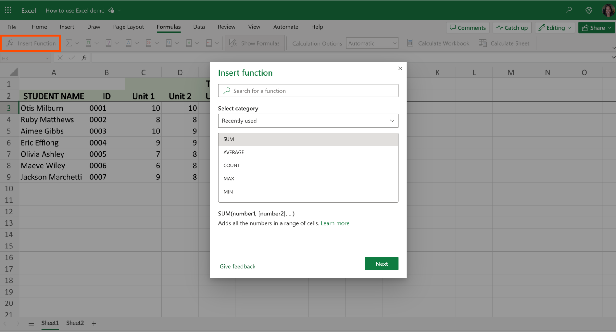
Select the function you want to use, and then click Next.

Here's a quick overview of the most common basic functions in Excel.
SUM: adds all the values in a cell range. For example,
=SUM(C3:G3)in our grade sheet would result in (aka return) the sum47.AVERAGE: returns the average of a range of cells. For example,
=AVERAGE(C3:G3)would return9.4.COUNT: counts the number of cells in a given range that contain numbers. For example,
=COUNT(C3:C9)would return7because every cell in that range contains a number. If, say, I deleted the value in cell C4, the count would automatically change to6.MAX: returns the highest value in a cell range. For example
=MAX(C3:C9)would return10.MIN: returns the lowest value in a cell range. For example,
=MAX(C3:C9)would return6.
To learn more, here's a comprehensive breakdown of every Excel function.
Now let's get back to how to use formulas in Excel.
To create a formula to calculate simple arithmetics, like adding, subtracting, or multiplying, you need to use specific symbols.
To add: use the
+sign.To subtract: use the
-sign.To multiply: use the
*sign.To divide: use the
/sign.To use exponents: use the
^sign.
Remember: to enter any formula in Excel, it must begin with = immediately followed by the formula. By default, Excel will use PEMDAS to determine the order of operations (what to calculate and in what order): Parentheses first, followed by Exponents, Multiplication, Division, Addition, and then, finally, Subtraction.
For example, if I enter =10-5*2, Excel will return 0. But if I enter =(10-5)*2, it'll return 10.
If you have a series of calculations that need to happen in a specific order, use PEMDAS.
Note: You can enter the cell name to add it to your formula, or you can click the desired cell to add it to your formula.
How to create charts and pivot tables
Now that you know how to create a worksheet, add data, and use formulas, let's kick things up a notch. Here, I'll cover more advanced ways to manipulate and visualize your data.
How to use charts in Excel
Let's say I want to quickly visualize how a student is performing from test to test. One way to do this would be to create a chart.
Highlight the data you want to include in your chart. In this example, I've selected the cell range
A2:G9. Note: a cell range spanning rows and columns is indicated by[top-left cell name]:[bottom-left cell name].From the ribbon, click Insert.
Click the Clustered Column icon, which looks like a vertical bar graph. To use a different chart type, click the Charts dropdown and select a different style.

The chart will appear directly in your spreadsheet—usually (and inconveniently) on top of your source data. To move it, click anywhere within the chart, and drag it to another area of your spreadsheet.

How to edit charts in Excel
To modify the data used to populate a chart, right-click it, and then click Select Data. Or, if you want to modify the chart formatting, click Format. The source data is fine in this example, but let's update the chart title (click Format).

In the Chart side panel that appears, you can edit every chart element, including the chart title, legend, and axes. Note: The chart elements vary depending on the chart style selected.
In this example, all I want to do is update the chart title. Click the down caret (⋁) beside Chart Title. In the Chart Title field, edit the chart name. In this case, I've changed it to Student grades by test. You can also change the position of the chart title. Or you can click the toggle beside Chart Title to hide the title altogether.

If you want to change the chart's source data, you can click Data in the side panel to toggle to that editor.
How to use pivot tables in Excel
A pivot table can be used to analyze massive amounts of data. With a pivot table, you can use the same data, manipulate it however you want, and get new insights each time—you don't have to create a new spreadsheet for each analysis. For spreadsheet power users, pivot tables are their bread and butter.
We have an in-depth tutorial on how to use pivot tables in Excel, but here's a quick overview.
Select all of the cells with source data that you want to use (including column headers).
From the ribbon, click Insert.
Click PivotTable.
In the Insert PivotTable side panel that appears, you have a couple options: Create your own PivotTable or use a recommended pivot table. Whether you create a new pivot table or use a prebuilt one, you can always modify it later on. For this example, we'll create a new one. In the Create your own PivotTable option, click New sheet.
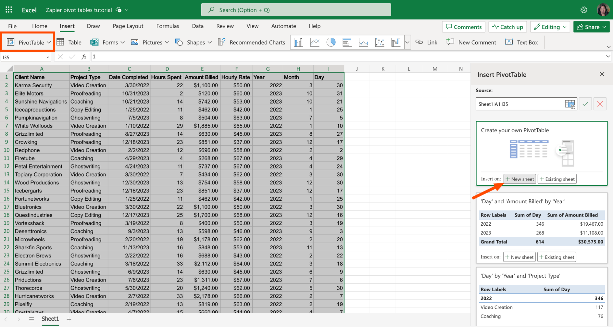
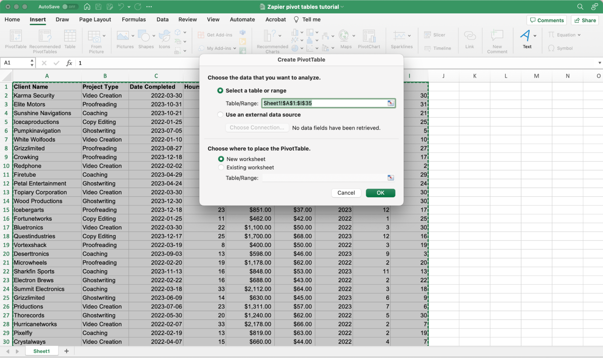
In the desktop app, Excel doesn't provide pivot table recommendations. Instead, in the Create PivotTable popup that appears, you can only choose the data you want to analyze and where to place your pivot table.
The pivot table always starts out empty. To build it out, use the PivotTable Fields editor in the side panel. You can click on fields (columns of data grouped by headers from the source data), and Excel will automatically add them to areas (Filters, Rows, Columns, and Values). Or you can drag and drop them into your desired areas to build a specific report.


In the example below, I created a pivot table to answer this question:
How much did we bill in 2023 for each client across different project types?

Pivot tables work similarly across spreadsheet apps. Here's how to use pivot tables in Google Sheets.
How to collaborate in Excel
Need to crunch numbers as a team? Or ask questions about specific points of data? Excel makes it easy to collaborate on a workbook.
How to add comments in Excel
If you want to leave a comment about a specific cell or range of cells, here's how.
Select the cell or cell range in the spreadsheet.
From the ribbon, click Comments.
In the Comments side panel, click New.
Enter your message in the comment box.
You can also tag other people directly in the comments by entering
@immediately followed by their name or email address. Note: This only works if the spreadsheet is stored in a SharePoint library or OneDrive for work or school.Click the Post comment icon, which looks like a right-facing arrow. Or use the keyboard shortcut
command+returnon a Mac orCtrl+Enteron Windows.

How to view and resolve comments in Excel
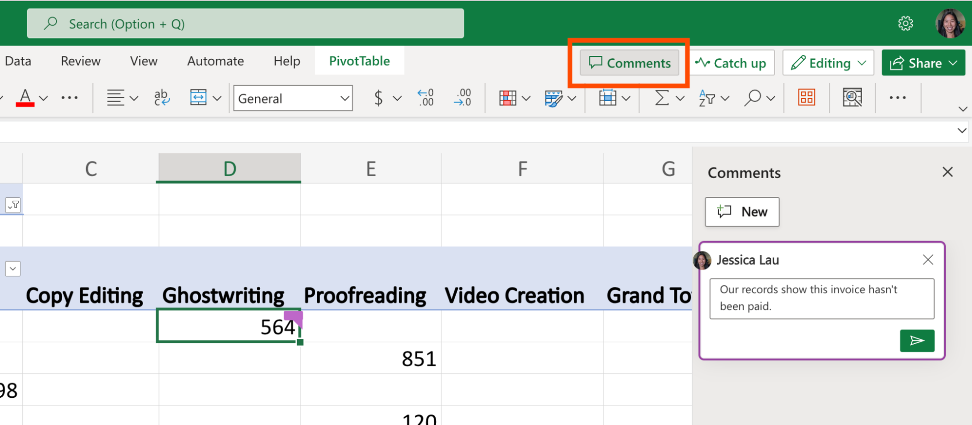
Once a comment is added to a cell, the upper-right corner of the cell gets flagged.

It's easy to miss the flag, though, especially if you're working with a lot of data. The best way to make sure you see all the comments in a spreadsheet is to open the Comments side panel (click Comments in the ribbon).

To respond to a specific comment, enter your message in that comment's message box. This will create a threaded response. You can also click the More thread options icon, which looks like an ellipsis (...), to take other actions:
Link to comment
Edit comment (if you posted the comment)
Resolve thread
Delete thread

How to share an Excel spreadsheet
Excel online offers a number of ways to share a workbook. In the ribbon, click Share.

From here, you have a few options:
Share. This lets you share your workbook with specific people by entering their names or email addresses. You can also limit their access to Can edit or Can view. Once you add their names or emails, click Send. This will notify your recipients that they now have access to your workbook.
Copy Link. This automatically copies your workbook link to your clipboard. Paste it as you normally would in a message to share the link.
Copy Link To This Sheet. If your workbook contains multiple sheets and you want to direct someone to a specific sheet, this option copies a link to that specific worksheet to your clipboard. Paste it as you normally would in a message to share the link.
Let's say you previously shared your workbook with a colleague, but they could only view the workbook—not edit it. If you want to update their access so they can also edit (or vice versa), here's how.
Click Share.
Click Manage Access.
Click the user whose permissions you want to update.
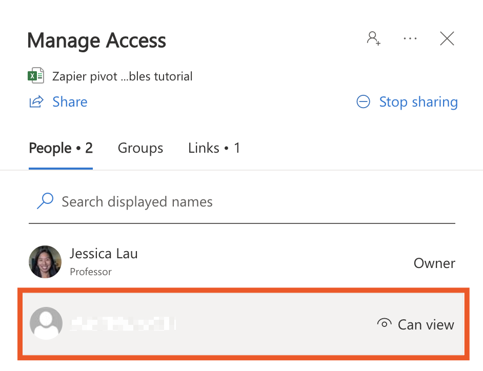
In the section Ways this person has access, click on their access type. This will look different depending on what access each recipient has.
Click the access type dropdown, and then select the desired access type.
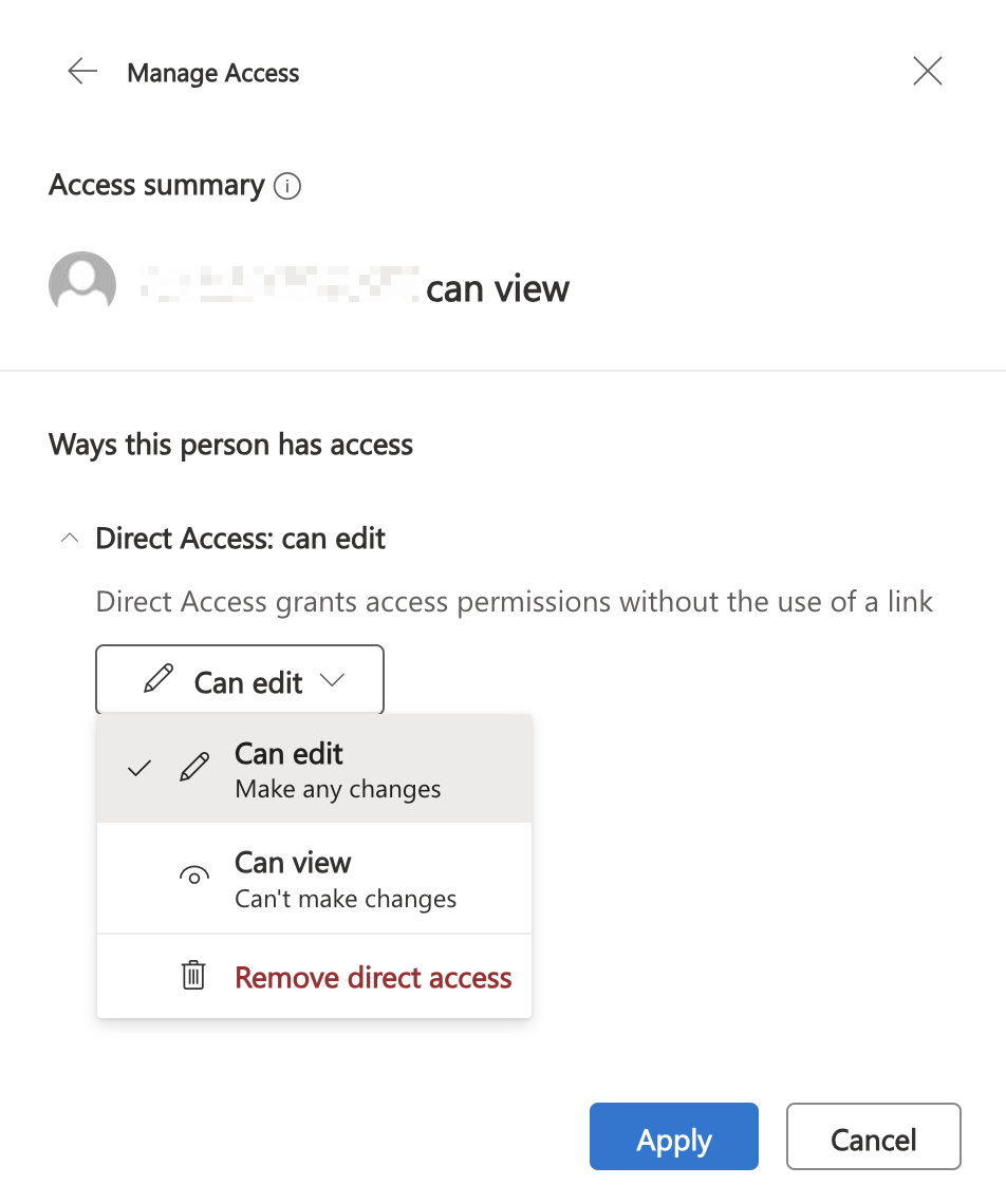
Click Apply.


That's it.
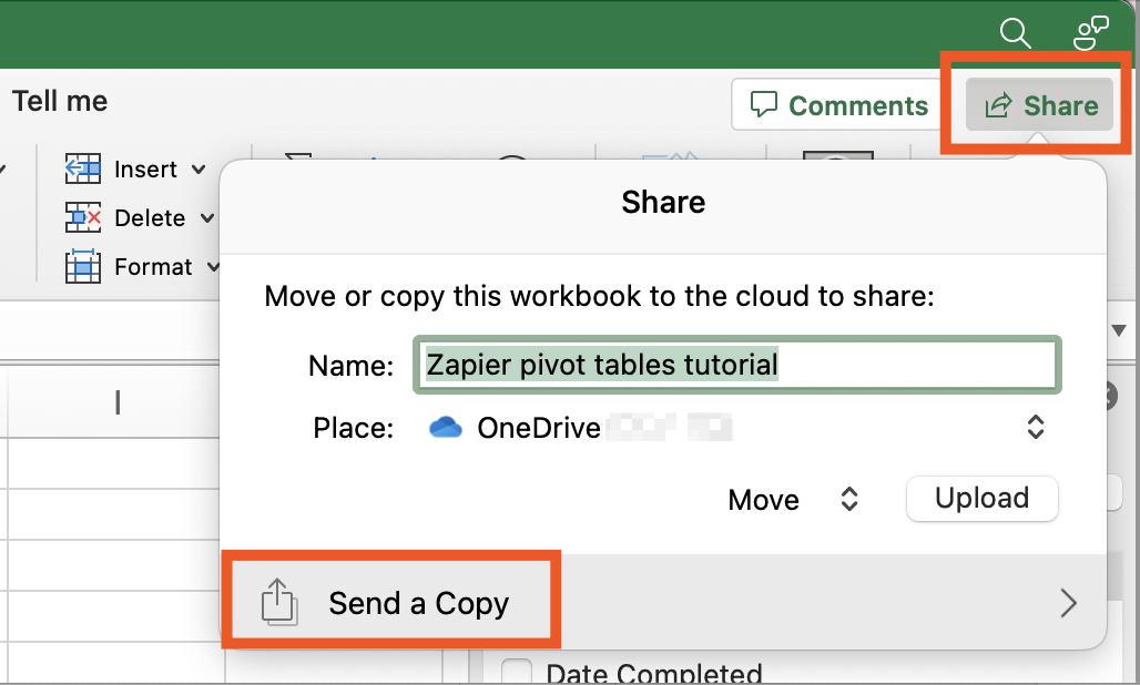
If you want to share a workbook created in the desktop app, Excel will prompt you to first move or copy your workbook to the cloud. If you don't have a cloud storage app, you can send a copy of the workbook via email directly through the app.
Click Share.
Click Send a Copy.
Click Email as Attachment.
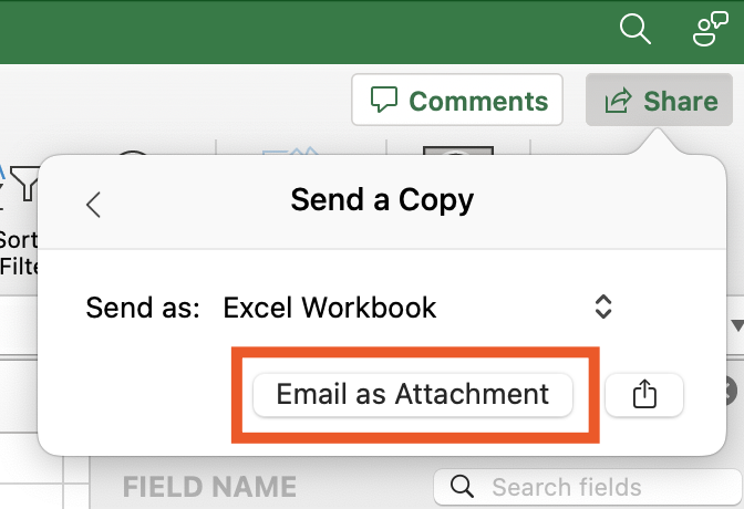


This will open a message box with your associated email app, complete with the workbook already added as an attachment. Send your email as you normally would, and you're all set.
Bonus: more Microsoft Excel tips and tricks
We've barely scratched the surface of what's possible with Excel, but it's a good start. As you play around with Excel spreadsheets, you may want to take a hands-off approach to formatting data—that's where conditional formatting comes in handy. Or you may run into the dreaded #VALUE or #REF error messages.
Here are some more Excel tips and tricks to keep handy:
Automate Microsoft Excel
Manually adding data to Microsoft Excel can be a real snooze—and it's ripe for human error. With Zapier, you can connect Excel to your go-to apps so you can automate spreadsheet-related tasks. For example, you can automatically add new form submissions to an existing workbook. Learn more about how to automate Excel, or get started with one of these workflows.
Add new Jotform submissions to Excel spreadsheet rows
Add new Jotform submissions to Excel as rows in a table
Add new Jotform submissions to Microsoft Excel as rows
Zapier is the most connected AI orchestration platform—integrating with thousands of apps from partners like Google, Salesforce, and Microsoft. Use forms, data tables, and logic to build secure, automated, AI-powered systems for your business-critical workflows across your organization's technology stack. Learn more.
Related reading:
How to find records in Google Sheets, Excel, and across apps
How to add new leads to a spreadsheet or database automatically
How to use Excel for project management (with 11 free templates)
This article was originally published in September 2016 by Matthew Guay. The most recent update was in July 2024.