When you're staring at endless rows of data in a spreadsheet, it can be hard to make sense of what it all means. And if you're scrambling to put together a presentation on the key takeaways from that spreadsheet—forget about it.
That's why I use conditional formatting. It lets you format rows and columns, which not only makes large data sets less of an eyesore but also makes your spreadsheet easier to digest.
Here's a step-by-step guide for how to use conditional formatting in Excel.
Table of contents:
Here's the short version of how to use conditional formatting in Excel (keep scrolling for detailed steps with screenshots).
Select the cell range that you want to apply conditional formatting to.
In the Home tab of your ribbon, click Conditional Formatting, and then select New Rule.
In the Conditional Formatting panel, select the rule type and customize the condition.
Select the formatting style.
Click Done.
Need a refresher on how to use Excel? Check out our beginner's guide to Excel.
What is conditional formatting in Excel?
Conditional formatting in Excel is a built-in feature that lets you dynamically format a cell's background and text style based on custom if/then rules that you set. For example, if the cell is blank, then add a yellow color fill to the cell.

Elements of conditional formatting in Excel
There are three key components that make up every conditional formatting rule:
Range: A range can be anything from a single cell to multiple cells across different rows and columns. The range indicates which cell(s) the rule applies to. In the example above, the range is C3 to C14.
Condition: This is the "if" part of the if/then rule. You can choose from more than a dozen options, including greater than, less than, between, and so on. In the example above, the condition is "if the cell contains a blank value."
Formatting: This is the "then" part of the if/then rule. It refers to the formatting that should apply to any given cell if the conditions are met. In the example above, the style is "fill with yellow."
How to use conditional formatting in Excel
Here's how to use conditional formatting rules in Excel. For this tutorial, I'll show you how to create a conditional formatting rule to easily identify which employees sold more than 140 units last year in our example spreadsheet.
A few notes to keep in mind:
This tutorial shows you how to add and modify conditional formatting rules primarily from the Conditional Formatting side panel. But you can kick off a lot of these rules from the Conditional Formatting dropdown in the ribbon.
If you add more than one conditional formatting rule to a given range, Excel will run through each rule in the order they were created. But once a rule is met by any given cell, subsequent rules won't override it.
I use the web version of Microsoft Excel, but the steps are pretty much the same in the desktop app.
Now let's dive in.
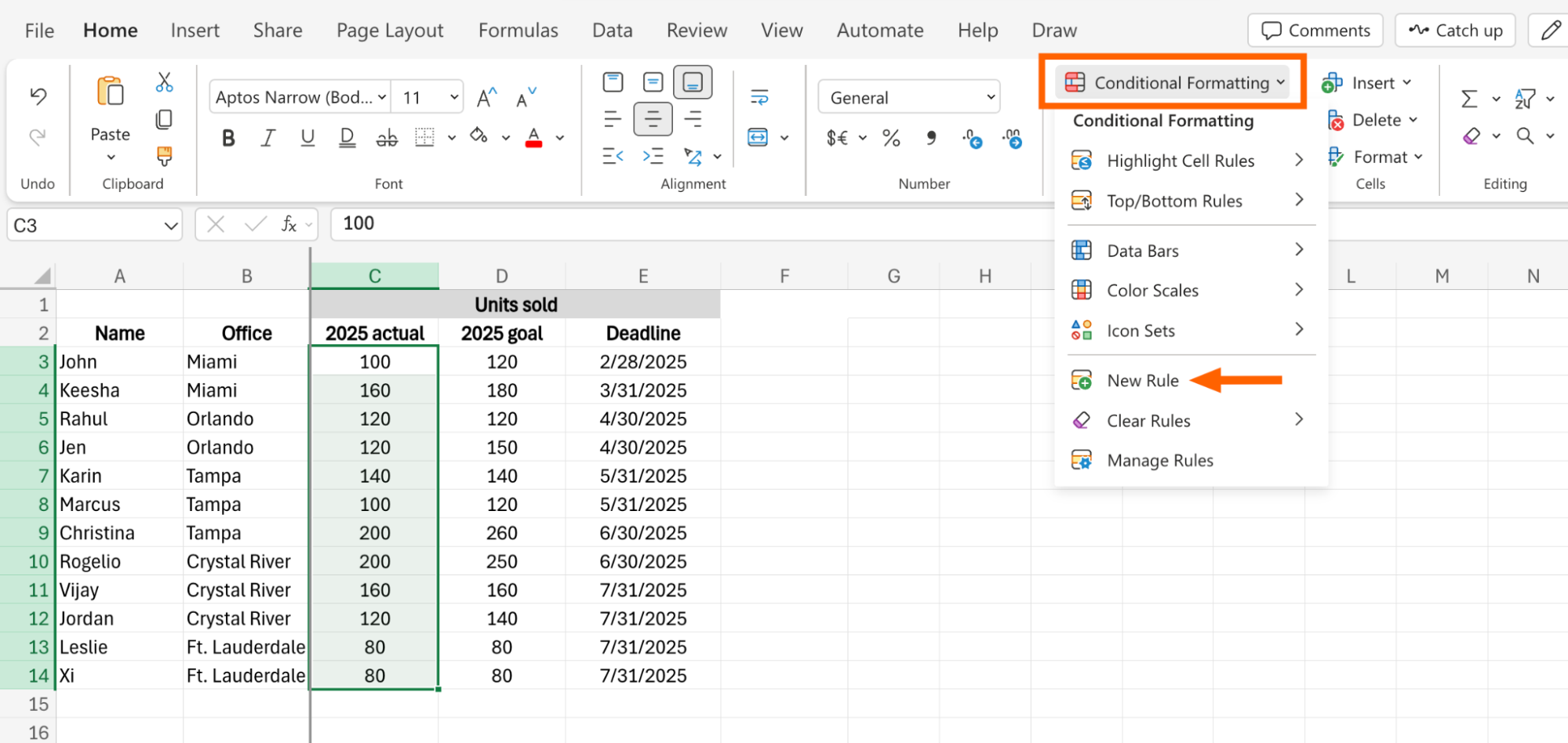
Highlight the cell range you want to apply your conditional formatting rule to. In this example, that's cells C3 to C14.
In the Home tab of the ribbon, click Conditional Formatting, and then select New Rule.
In the Conditional Formatting side panel, click the dropdown under Highlight cells with, and select Cell value.
Another dropdown will appear next to Cell value. Click it, select Greater than, and enter 140 in the value field.
Under Format Style, choose from one of the preset options, or click the Custom format icon, which looks like a plus sign (
+), to customize it.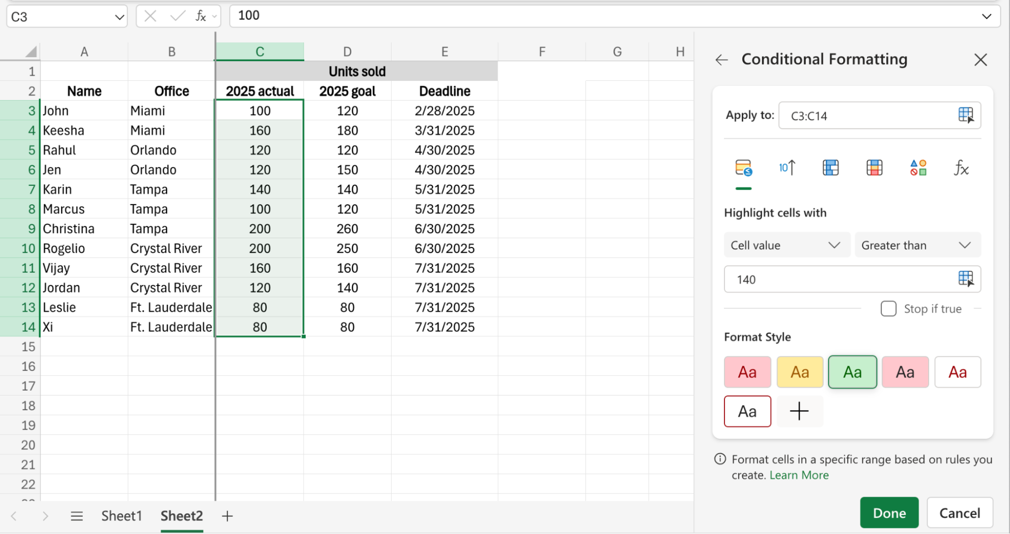
Click Done.
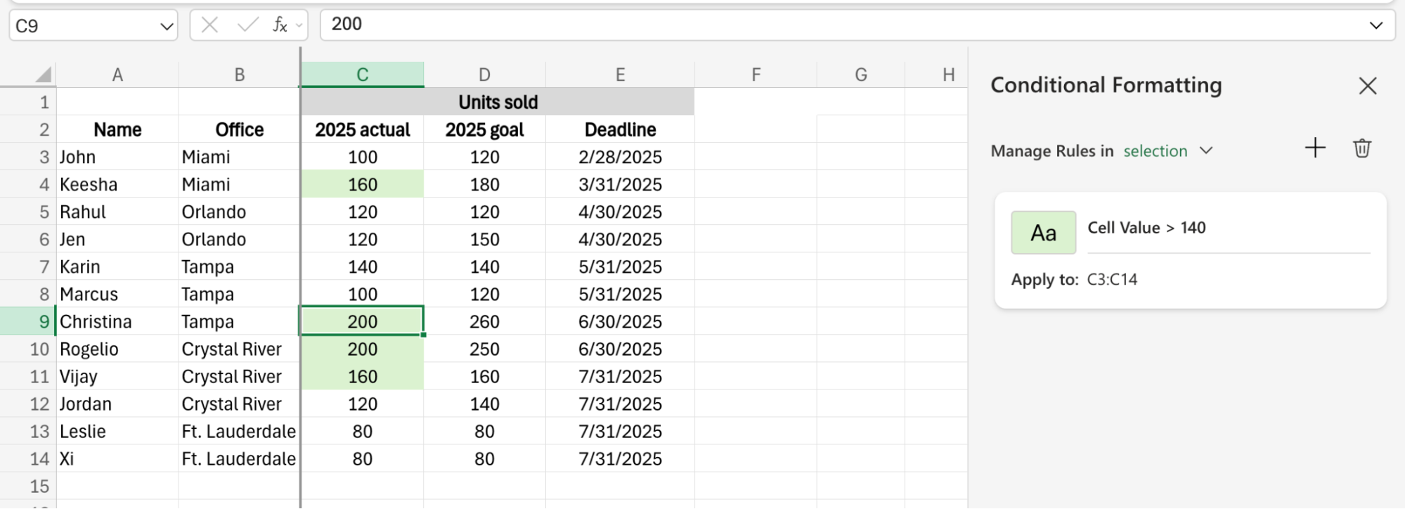


Now you can easily identify last year's overachievers.
How to remove conditional formatting in Excel
If you no longer want Excel to automatically format specific cells, here's how to remove conditional formatting in Excel.
In the Home tab of the ribbon, click Conditional Formatting, and then select Manage Rules.
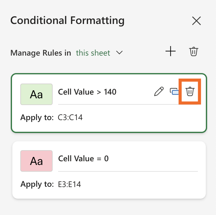
In the Conditional Formatting side panel, click the dropdown next to Manage Rules in, and select this sheet.
A list of all the conditional formatting rules for that sheet will appear.
Hover over the conditional formatting rule that you want to delete, and then click the Delete icon (it looks like a garbage can). Or, if you want to delete all your rules in one fell swoop, click the Delete icon next to Manage Rules in.

Conditional formatting in Excel: Rules and styles
Now that you know how to create conditional formatting rules in Excel, let's explore all the ways you can format your rules.
Highlight Cell Rules
This is the default conditional formatting rule in Excel. It allows you to highlight cells based on specific cell values. Common Highlight Cell Rules like Greater Than, Less Than, Between, and Equal to are self-explanatory, so here's a brief description of the last three available options:

Text that Contains. This rule highlights cells that contain particular text.
A Date Occurring. This rule highlights cells that contain a date from today, yesterday, last week, last month, and so on. It's a dynamic rule, which means that the cells that meet the condition will change relative to the current date.
Duplicate Values. This rule highlights repeat values within a given range. If you want to then delete the duplicates, here's how to remove duplicates in Excel.
Top/Bottom Rules
Top/Bottom Rules help you quickly highlight the best and the worst performers from a selected range—no complicated formulas required.

For Above and Below Average, Excel doesn't give you a way to specify the average. But rules like Top and Bottom 10 Items and Top and Bottom 10% can be modified. For example, if you want to view the top performing employees based on the number of units sold last year, you can modify this in the Conditional Formatting panel to show only the top three instead of 10.

Data Bars
Data Bars adds bar graphs in the background of each cell with each bar filled relative to other cells' values within the given range.

In the example below, I applied a data bar to the 2025 actual units sold cell range. The most number of units sold in this range is 200, so any cells containing this value show a bar graph spanning the entire cell. Meanwhile, cells containing half the max value—100 in this case—show a bar graph that runs halfway through the cell.

Color Scales
Color Scales automatically applies a color-based hierarchy system based on your conditional formatting rule.

There are multiple scale options available, so here's an example of how it works using the most commonly used option: Green - Yellow - Red Color Scale. When applied, it adds a green background to cells containing the highest values and a red background for cells containing the lowest. Cells containing values in between the highest and lowest are split using shades of orange and yellow.

Icon Sets
Icon Sets lets you add different icons—like arrows, stars, and flags—to each cell based on the cell's numeric value. Similar to Color Scales, it's dynamic so the icons will automatically update if the cell values are changed.

In the example below, I used the 3 Triangles icon set for cells C3 to C14. Cells containing the highest values have an up-facing green arrow; cells containing the lowest values have a down-facing red arrow; and cells containing in-between values have a light-orange bar.

How to use conditional formatting in Excel with Copilot
If clicking through a few menus is what pushes you over the how-is-it-only-Tuesday edge, you can use Copilot, Microsoft's built-in AI assistant, to set conditional formatting rules up for you.
Before you get too excited, keep the following in mind:
You can use this feature only if you have a Copilot Pro subscription or a Microsoft 365 Personal or Family subscription that includes Copilot.
Copilot works only with Excel files stored on OneDrive or SharePoint with AutoSave turned on.
Be sure to format your data as tables—Copilot doesn't work with regular ranges.
If those don't make you reconsider how much time Copilot really saves you for setting up conditional formatting rules (it doesn't, in my opinion), then here's how to use it:
Click Copilot on the ribbon to open a new chat. Or click any cell, and select the Copilot icon that appears next to it.
Describe what you need in the message bar. For example, "Fill the top three values in column C with the color yellow." The more specific your AI prompt, the better.
Copilot will generate a conditional formatting rule, along with a preview of the results, and display it in the chat.
If the preview looks good, click Apply.
Automate Microsoft Excel
Now that you know how to make your spreadsheet easier to digest, it's time to streamline your Excel-related tasks. By pairing Excel with Zapier, you can turn Excel into your source of truth and connect it to all the other apps you use. Automatically log form submissions, notify your team about updates to a spreadsheet, and build fully automated systems for your data.
Learn more about how to automate Excel, or get started with one of these pre-made workflows.
Add new Jotform submissions to Excel spreadsheet rows
Zapier is the most connected AI orchestration platform—integrating with thousands of apps from partners like Google, Salesforce, and Microsoft. Use forms, data tables, and logic to build secure, automated, AI-powered systems for your business-critical workflows across your organization's technology stack. Learn more.
Related reading:
This article was originally published in July 2019 by Khamosh Pathak. The most recent update was in May 2025.