When you're staring at endless rows of data in an Excel spreadsheet, it's easy for all that information to turn into one blurry mess. Then there's the matter of extracting specific data. In addition to spending what feels like an eternity scrolling through the spreadsheet to find what you need, you then second-guess if you actually pinpointed the right data.
That's where VLOOKUP in Excel comes in: it takes the guesswork out of finding and retrieving data in spreadsheets.
Here's the short version of how to use VLOOKUP in Excel (keep scrolling for more details).
Click the cell where you want Excel to return the data you're looking for.
Enter
=VLOOKUP(lookup value,table array,column index number,range lookup).Press Enter or return.
Table of contents:
Need a refresher on how to use formulas and functions in Excel? Check out our beginner's guide to Excel.
What is VLOOKUP in Excel?
VLOOKUP in Excel is a built-in function that searches for a value in one column based on a given value in another column. The formula is made of four parameters (or arguments):
Lookup value: This is the value you want Excel to search for. Note: The lookup value must be in the first column in the given range. For example, if your lookup value is in cell
A3, then your range should start withA.Table array: This is the cell range containing the lookup value and the value you want Excel to return (the data you're looking for).
Column index number: This is the column number in the given range containing the value you want Excel to return. If your table array is
A2:D10, for example, count columnAas your first column, columnBas your second, and so on. If your table array isC2:F10, count columnCas your first column, columnDas your second, and so on. Your column index number tells Excel which column to retrieve the data you're looking for.Range lookup: This is an optional parameter. By default, the VLOOKUP function always returns an approximate match (designated by
TRUE). If you want an exact match, enterFALSE.
Put those parameters together and you get this VLOOKUP formula:
=VLOOKUP(lookup value,table array,column index number,range lookup)
You can use the same function in Google Sheets to quickly extract information from complex datasets. Here's a step-by-step guide on how to use VLOOKUP in Google Sheets.
How to use VLOOKUP in Excel
Here's a detailed breakdown of how to use VLOOKUP (or vertical lookup). Note: I'm using Excel online, but the steps are the same in the desktop app.
To keep this tutorial simple, I'll show you how to use the VLOOKUP function in Excel to identify an employee's ID based on their last name—in this case, it's Kwon. While you'd probably use VLOOKUP for something more complex with a much larger dataset, the steps to use VLOOKUP remain the same.

A quick reminder: the lookup value must be in the first column of your table array. For this demo, our lookup value (Kwon in cell B6) will be in the first column of our table array (B2:D10). If you're working with a different dataset where the lookup value isn't in the first column, you may have to reorganize your data. Or you can copy and paste the columns you're working with into another area of your worksheet. If you go with the latter, I recommend pasting the data into a new worksheet altogether to keep your data manageable.
Once your data is organized, you're ready to get started.
Click the cell where you want Excel to return the data you're looking for. In this case, click cell B13.
Enter
=VLOOKUP.Press Enter or return. Excel will automatically add a left parenthesis after the function, so it looks like this:
=VLOOKUP(.Input the following parameters immediately after the parenthesis, separating each one with a comma.
Lookup value:
B6Table array:
B2:D10Column index number:
3(Remember: the value we want Excel to return [employee ID] is in column D, which is the third column of the given cell range.)Range lookup: Enter
FALSEto get an exact match
Enter the right parenthesis
)to close your formula so that cell B13 now reads=VLOOKUP(B6,B2:D10,3,FALSE).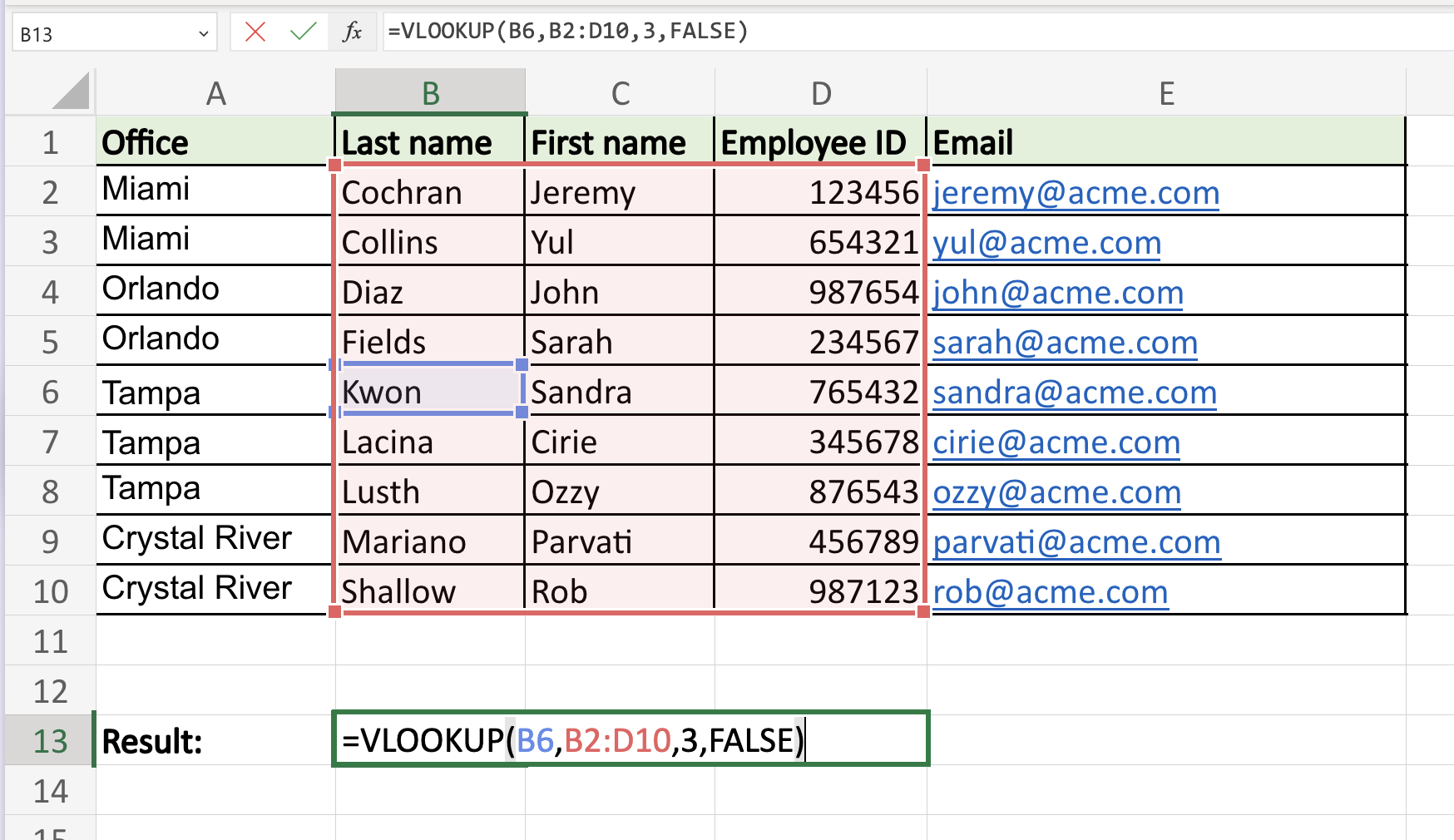
Press Enter or return.
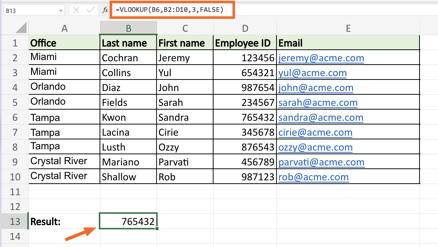


Excel immediately returns the corresponding value: 765432.
How to do VLOOKUP in Excel with two spreadsheets
Let's say Sheet 1 of our demo workbook is our primary spreadsheet—it contains every bit of employee data. There's also a second spreadsheet (Sheet 2), which contains only employee names and their updated company email addresses.

Now you need to update the email addresses in Sheet 1 with the new email addresses from Sheet 2. You can accomplish this with the VLOOKUP function, but you'll need to modify your table array parameter to tell Excel which spreadsheet contains the corresponding lookup value you want it to return.
This is the modified VLOOKUP formula to return a value from another sheet within the same workbook:
=VLOOKUP(lookup value,sheet!range,column index number,range lookup)
Let's use VLOOKUP to update the email address in cell E2 of Sheet 1 with the email address in cell C2 of Sheet 2.
Click cell E2 of Sheet 1.
Enter
=VLOOKUP(B2,Sheet2!$A$2:$C$10,3,FALSE). Here's a breakdown of the modified table array:Sheet2!: This is the name of the spreadsheet that contains the given cell range. Note: to reference another worksheet, input
[name of sheet]!. If your sheet name contains spaces or non-alphabetical characters, it must be enclosed in single quotation marks. For example,'Sheet 1'!.$A$2:$C:$10: The cell range is A2:C10. To prevent the range from changing when copying the formula to other cells, we lock it in using absolute cell references.
Press Enter or return.

Excel returns the corresponding value from Sheet 2 in cell E2 of Sheet 1: j.cochran@acme.com.
To quickly update the remaining email addresses in Sheet 1, drag the fill handle from cell E2 down.

How to do VLOOKUP in Excel with two workbooks
To use VLOOKUP to retrieve data from another workbook, all you have to do is include the file name of the other workbook within square brackets immediately followed by the sheet name and table array. Here's the formula template:
=VLOOKUP(lookup value,[file_name.xlsx]Sheet!range,column index number,range lookup)
Let's say we stored the employees' updated email addresses in Sheet 1 of the 2023_employee_emails.xlsx workbook instead. To populate the new email address in cell E2 of our primary spreadsheet, enter:
=VLOOKUP(B2,[2023_employee_emails.xlsx]Sheet1!$A$2:$C$10,3,FALSE)
How to use VLOOKUP in Excel with Copilot
If you've made it this far without rage-quitting Excel and going to live off the grid in Saskatchewan, I have a reward for you: you can use Copilot, Microsoft's built-in AI assistant, to build the VLOOKUP formula for you.
Before you get too excited, keep the following in mind:
You can use this feature only if you have a Copilot Pro subscription or a Microsoft 365 Personal or Family subscription that includes Copilot.
Copilot works only with Excel files stored on OneDrive or SharePoint with AutoSave turned on.
Be sure to format your data as tables (Copilot doesn't work with regular ranges).
Now, let's dive in.
With your workbook open, click Copilot on the ribbon to open a new chat. Or click any cell and select the Copilot icon that appears next to it.
Describe what you need in the message bar. For example, "Write a VLOOKUP formula to pull email addresses from Table A to Table B." The more specific your AI prompt, the better.
Copilot will generate a formula, along with a preview of the results, and display it in the chat.
Optionally, prompt Copilot to tweak the formula until it's exactly what you need.
Hover over Insert column below the results preview to view the results directly in your sheet. If it looks good, click Insert column. Alternatively, you can copy and paste the formula yourself.
It's that easy. Just don't tell your past self, who's still weeping into a spreadsheet in 2013.
Automate Excel with Zapier
Manual data entry doesn't scale—and it's easy to get wrong. With Zapier as an orchestration layer, you can connect Excel with thousands of other apps and orchestrate how data flows across your tech stack. For example, automatically log new event feedback in Excel, use AI to categorize the feedback type and analyze customer sentiment, and send a summary of the analysis to your team in Slack or via email.
Learn more about how to automate Excel, or try one of these pre-made templates to get started.
Add new Typeform entries as rows on an Excel spreadsheet
Add new Jotform submissions to Excel spreadsheet rows
Zapier is the most connected AI orchestration platform—integrating with thousands of apps from partners like Google, Salesforce, and Microsoft. Use forms, data tables, and logic to build secure, automated, AI-powered systems for your business-critical workflows across your organization's technology stack. Learn more.
Related reading:
This article was originally published in July 2019 by Khamosh Pathak. The most recent update was in August 2025.