We independently review and test every app we write about. When you click some of the links on this page, we may earn a commission. Learn more.
Full disclosure: You can ask Google Sheets' built-in AI assistant Gemini to write a VLOOKUP formula for you and save yourself from reading the rest of this article.
But there's something deeply unsettling about having a robot paste a formula into your spreadsheet and having no idea how it works. It's like letting a robot vacuum clean your apartment. It'll probably do a great job, but you won't know until your dog starts barking from the room the robot accidentally trapped it in.
So here's your chance to actually learn how to use VLOOKUP in Google Sheets. Plus, what it does, how it works, and how to bend it to your will. That way, when Gemini gets it wrong (it happens), you'll know exactly how to fix it.
You can make a copy of our demo spreadsheet to follow along as I walk you through the tutorial.
Table of contents:
What is VLOOKUP in Google Sheets?
VLOOKUP in Google Sheets is a function that searches for a specific value in one column of a table and returns a corresponding value from another column in the same row. It's especially useful when you're working with large datasets—for example, a spreadsheet with thousands of employee names and ID numbers—and you need to pull specific information into another part of the spreadsheet, like an organizational chart or a performance review.
Here are the components that go into the function:
Table: You have a table with rows and columns of data.
Value: You know a specific value, like a name or ID, and you want to find more related information.
Lookup: You use VLOOKUP to look for that value in the same row but a different column.
Retrieve: Once it finds the value, VLOOKUP gives you the information.
Think of it like looking up a name in a phone book (remember those?). You find the name you're searching for, and you can see the phone number right next to it. VLOOKUP does the same thing with data in Google Sheets.
VLOOKUP formula: syntax and inputs
The VLOOKUP formula tells Google Sheets what value to search for, where to look, and what to return. Here's the formula:
=VLOOKUP(search_key, range, index, [is_sorted])
Here's what each of those inputs means:
search_key: This is the value you're looking for in your table.
range: This is the area you want to search for your value, or the section of your table where you think you'll find the information. It has to be at least two columns.
index: This is a column number within the range you provided where your desired data is located. For example, if you're looking up names and you want corresponding ages, the column number where ages are listed would be your index.
is_sorted: This tells VLOOKUP if the data in the range is sorted in ascending order (TRUE) or not (FALSE).
If you set it to TRUE, Google Sheets will assume the data is in ascending order (A to Z or smallest to largest) and can search faster. But this also means it will search for a close but not exact match. So it'll find the closest value that's less than or equal to the lookup value.
If you set it to FALSE, Google Sheets will search more thoroughly for an exact match. If VLOOKUP doesn't find an exact match, it'll return an #N/A error.
How to use VLOOKUP in Google Sheets
The absolute simplest way to use VLOOKUP in Google Sheets is by asking Gemini to use it for you. Just describe what you're trying to do in plain English, and it'll handle the rest.
Here's an example of me asking Gemini to use VLOOKUP to quickly do what I'm about to show you in painful detail how to do manually:

But if you didn't come here just to let a robot do your job for you, congratulations—you still have a will to learn. Here's the step-by-step breakdown.
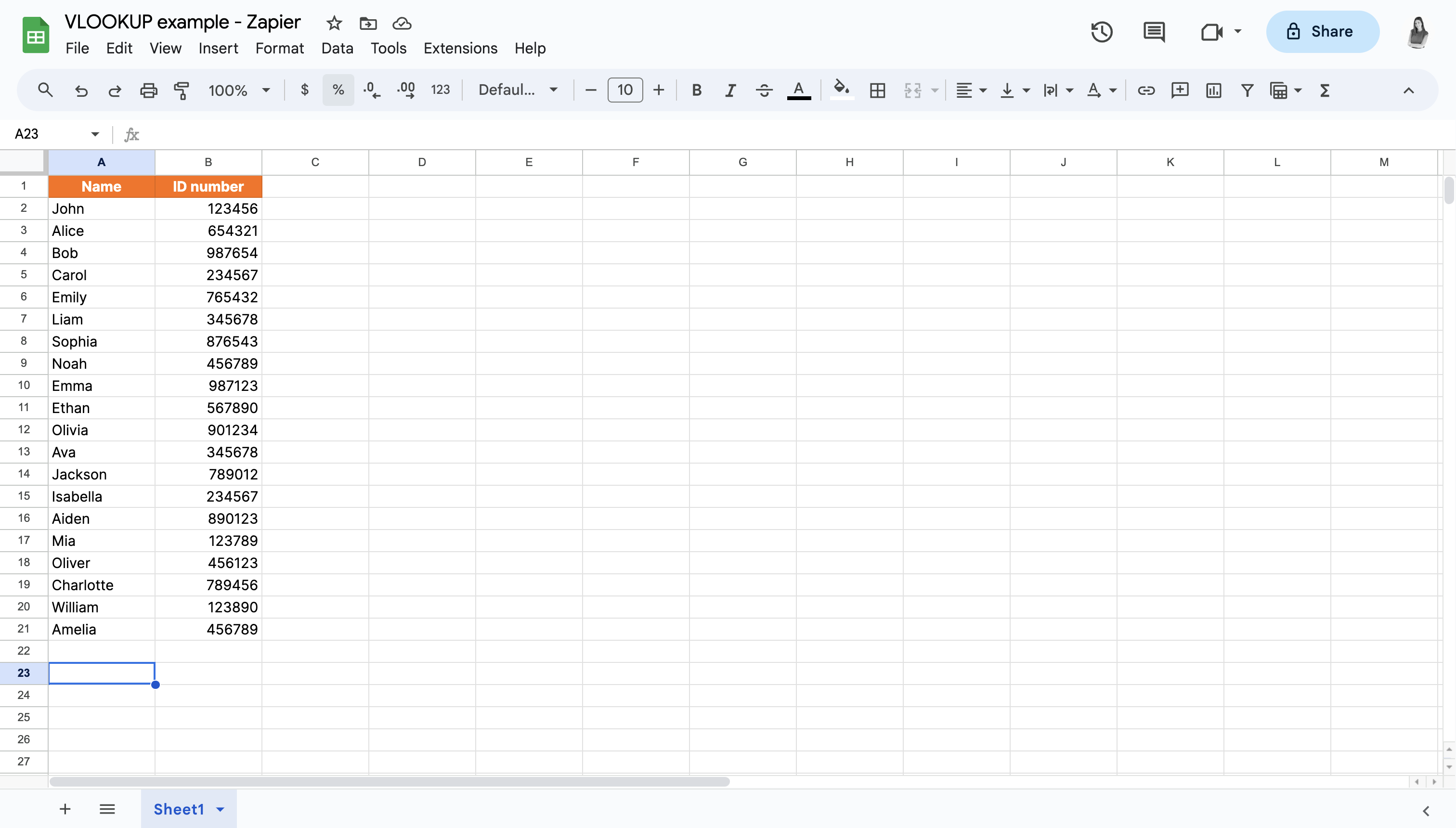
Note: If you needed to use VLOOKUP in real life, you'd probably be dealing with a much larger and more complex dataset. But for the sake of learning how to use the function, I'll keep our example super simple with a small list of pretend employees and ID numbers. Our goal is to find the ID number of a specific employee.
Follow along in the demo spreadsheet under the "Simple example - FALSE" tab.
Organize your data. Enter your data into a spreadsheet or locate an existing table. (The data is already there for you in this spreadsheet.)
Select an output cell. Click the cell where you want the information you're looking for to end up. In this case, click into cell A23.
Enter the VLOOKUP function. Enter the VLOOKUP function into that cell:
=VLOOKUP(search_key, range, index, [is_sorted])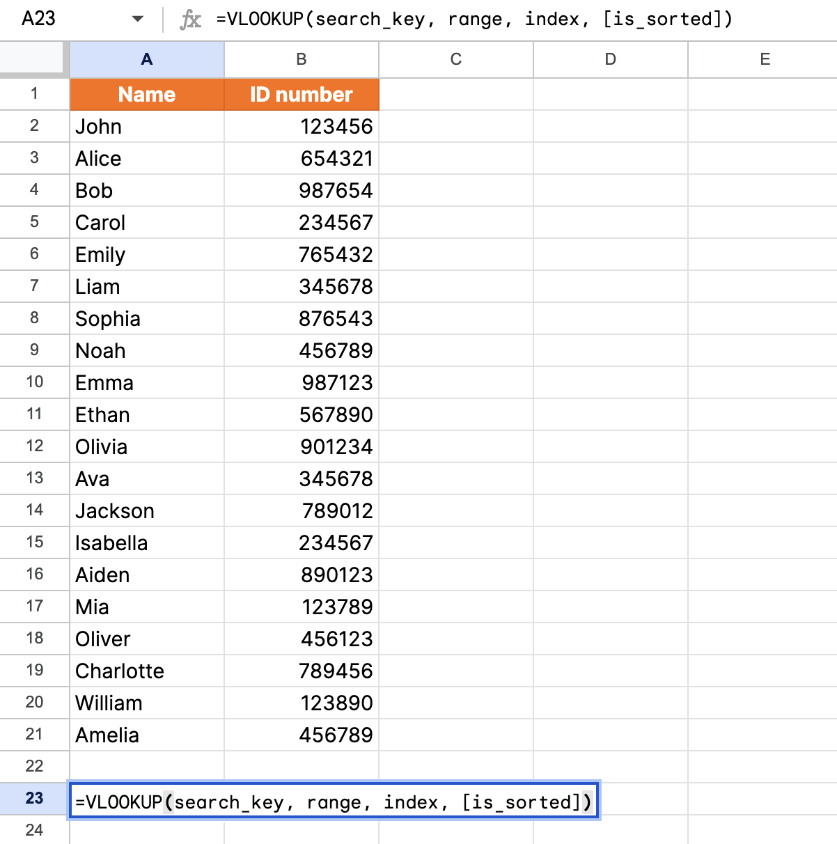
Enter the search_key. Replace the search_key with the name of the employee you're looking for. We'll look for Mia in this example, so we want to enter
A17as the search key.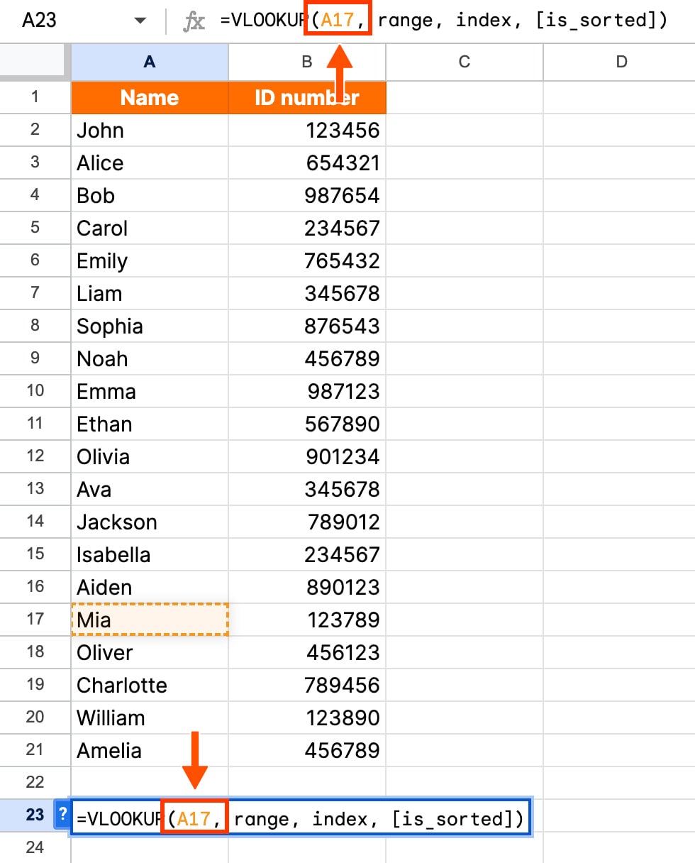
Set the value range. Now we'll replace the range with the cells that contain the data we want to search. In this case, our data is in columns A and B, so we'll replace range with
A:B.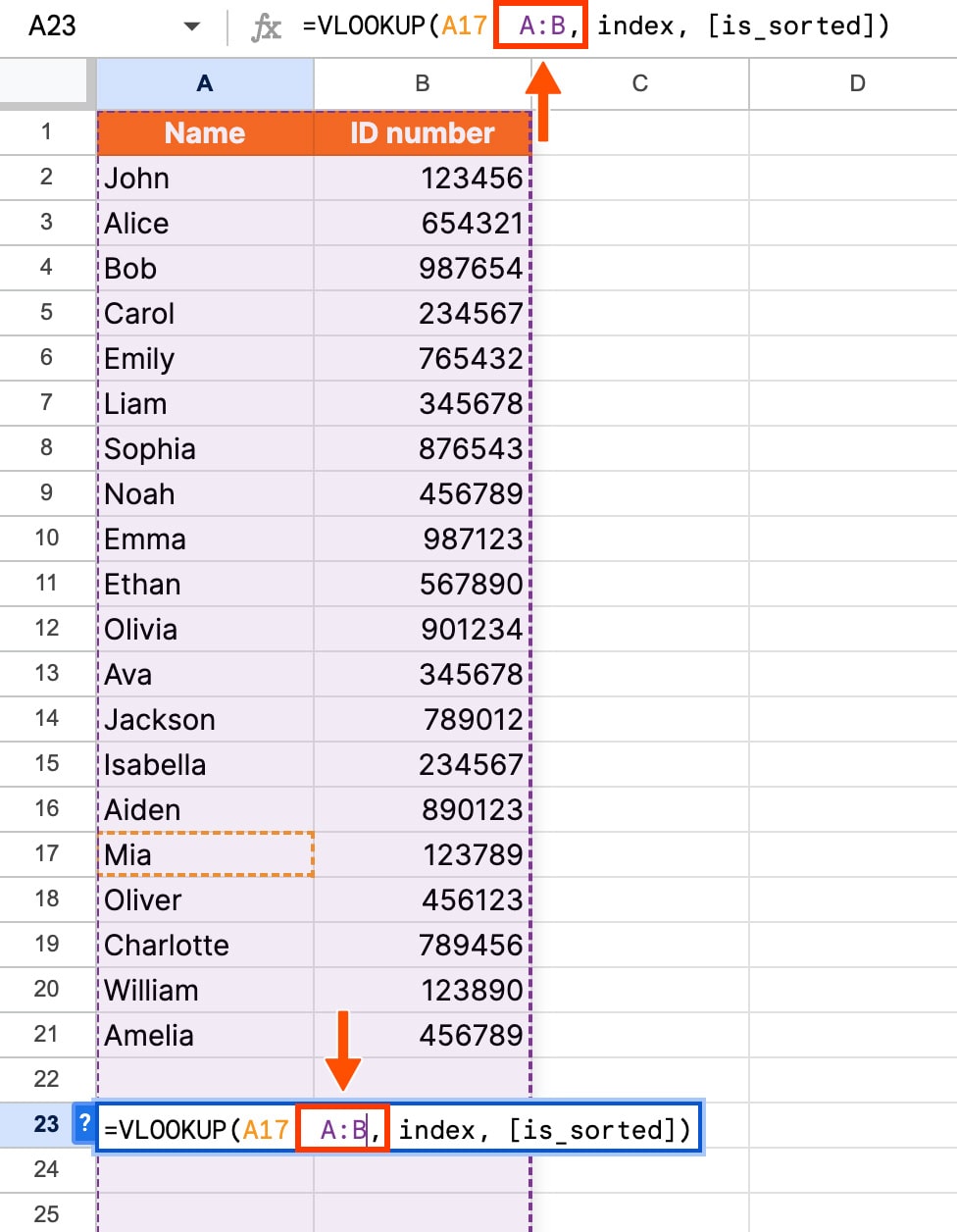
Set the index column. Next, replace index with the column number that contains the data you want. To find the index column, count from the leftmost column. We need information from the ID number column, which is the second column from the left. So we'll enter
2for index.
Determine is_sorted value. In our example, the data isn't sorted in order, so we'll need to use
FALSEfor [is_sorted].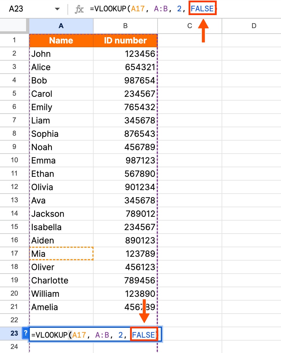
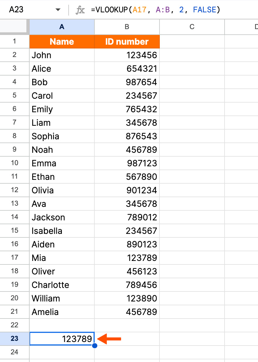
Execute the function. Once you've entered all your inputs, hit Enter. If you did everything right, the function should return the value you were looking for. In our case, it returned Mia's employee ID number: 123789.


Why is VLOOKUP not working in Google Sheets?
Is VLOOKUP not behaving like it's supposed to in Google Sheets? No one's surprised. Here are a few common errors you'll almost definitely encounter and how to fix them.
VLOOKUP returns an unexpected value
If your VLOOKUP function returns a value you weren't looking for, double-check your formula. This can occur if [is_sorted] is set to TRUE, but the first column in the selected range isn't sorted numerically or alphabetically in ascending order. To troubleshoot, change [is_sorted] to FALSE.
VLOOKUP only returns the first matching value
By design, VLOOKUP in Google Sheets always returns the first result found. If you have multiple matched search keys, you'll need to assign them unique values so VLOOKUP can search for them properly.
VLOOKUP with unclean data
VLOOKUP in Google Sheets may not work properly if you're searching for values with extra spaces or other typographical errors. Be sure to remove unwanted spaces in your sheet. You can start by going to Data > Data Cleanup > Trim whitespace.
VLOOKUP returns #N/A error
This error can occur if you use VLOOKUP in Google Sheets to look up a value for which no exact match exists in your first column.
How to VLOOKUP across multiple sheets
Let's say you want to see how many products a customer purchased, but you have multiple customers with the same name (looking at you, Tim Johnson). Normally, the VLOOKUP function is limited to one search value, but you can scan for multiple criteria with a bit of extra legwork. Here's how it's done:
Insert a new "helper" column to the left of your lookup columns. This will be the leftmost column in your table.
In the first cell of this column (A2 if your data starts in row 2), enter the formula
=B2 & " " & C2. This will join the values in your existing columns and separate them with a space.Copy that formula to the rest of the cells in the helper column.
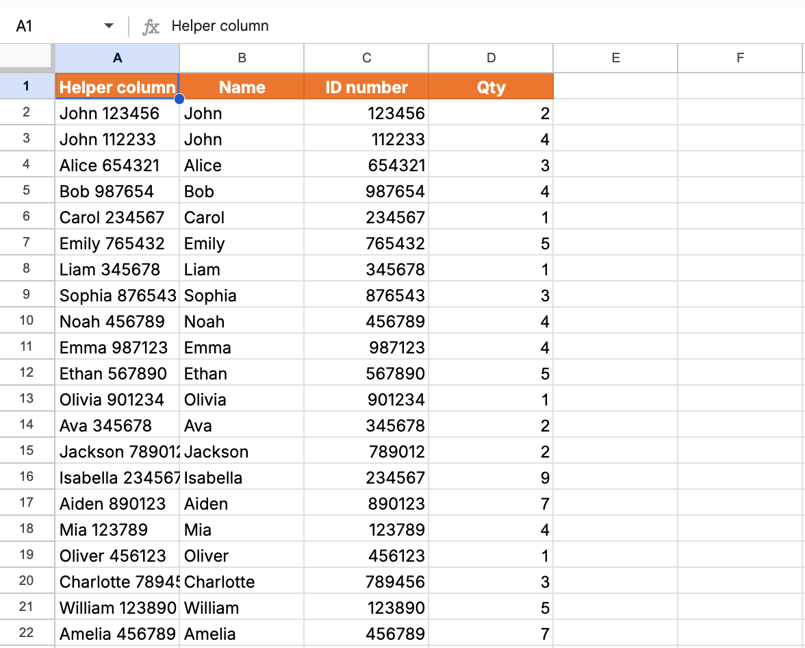
Using the standard VLOOKUP formula, place both criteria you want to search for in the lookup_value argument, separated with a space. In my example, I want to search for someone named John with the ID number 112233. Here's the formula I used:
=VLOOKUP("John 112233", A2:D22, 4, FALSE)The formula will return a value based on your search criteria (the quantity 4, in my example).
You'll need to replace A2:D22 with the actual range of your table, including the helper column. The number 4 indicates that you want to return the value from the fourth column in the table. You can also adjust this as needed.

6 more tips for using VLOOKUP in Google Sheets
If you're like me and need a real human to hold your hand through the process (bye, Gemini), here are some additional pointers for using VLOOKUP.
1. Keep your data organized
Organized data reduces the chances of errors in your VLOOKUP formulas. Here are a few tips.
Use headers. Clear, descriptive headers for your columns makes it easier to understand what each column represents. Then, when you perform a VLOOKUP function, you can quickly see where you need to pull data.
Sort data. If you aren't looking for an exact match, you'll need to sort your data in ascending order so you can mark the is_sorted parameter as TRUE.
Eliminate empty cells. Empty cells within your dataset could lead to errors or incorrect matches.
2. Pre-sort the values in the leftmost column
One annoying quirk about the VLOOKUP function is that it can't look to the left. Before you start, make sure the column that houses your search_key is the leftmost column of your range.
Take our simple example from earlier. If we switch the order of the columns, with ID number coming before name, the function returns an error. This is because we selected B17 as our search_key and then asked it to pull data from the column to its left.

3. Use INDEX/MATCH for advanced functionality
But what if moving your columns would be a giant pain? Maybe it's a huge dataset or you have formulas in the spreadsheet that can't be moved around.
In that case, you'll want to ditch VLOOKUP and use INDEX/MATCH for more flexibility. That formula is: =INDEX(array or reference,MATCH(lookup_value,lookup_array,[match_type])
You can see this in action under the "INDEX/MATCH example" tab in our template.
For our same simple example, that formula would look like =INDEX(A2:A21,MATCH(B17,B2:B21,0))

Here's why:
The array or reference is the range where the data you're looking for could be. In our case, that's A2:A21 (the ID number column).
The lookup_value is your search_key, or the value you're looking for. That's B17 (Mia) in our example.
The lookup_array is the range where your lookup_value is located. That's B2:B21 (the name column) for us.
The [match_type] tells MATCH how to search. Use 0 for an exact match (that's what we want here: find the row that's exactly "Mia"). Use 1 if the lookup column is sorted in ascending order and you want an approximate match, or -1 if it's sorted in descending order.

4. Consider wildcard characters
You can use wildcards to perform partial matches with the VLOOKUP function. Wildcards are special characters that represent unknown or variable characters in a search pattern.
For example, an asterisk (*) can represent any sequence of characters, including no characters.
Check out an example of this under the "Wildcard * example" tab in our demo template. Suppose you have a list of ID numbers and employee names, and the first letter in each ID represents the employee department. You want to find the HR employee in the list whose ID number starts with H. You can use the * wildcard to perform this partial match.
You just need to replace your search_key with "H*". It would look like this: =VLOOKUP("H*",A2:B10,2,FALSE)

However, if your ID numbers only contain numbers, no letters, you'll need to use a different formula. Let's say ID numbers start with 4. Your formula would be: =VLOOKUP("4*",ArrayFormula(TO_TEXT(A1:B10)),2,FALSE)

5. Use FALSE to troubleshoot
Getting error responses or incorrect results? Try using FALSE in your is_sorted parameter to get exact matches first. If that doesn't help, then look into other reasons it didn't work.
6. Make VLOOKUP in Google Sheets case-sensitive
VLOOKUP is not case-sensitive, which means it doesn't pay attention to the difference between lowercase and uppercase letters. If that matters in your search, you'll need to use a separate formula: ArrayFormula(INDEX(return_range, MATCH (TRUE,EXACT(lookup_range, search_key),0)))
Automate Google Sheets with Zapier
If you followed all those instructions for using VLOOKUP in Google Sheets just to prove you're not entirely at the mercy of robots, honestly—respect. But just because you can use your human brain for the task, doesn't mean you have to.
When you use Zapier's Google Sheets integration, you can connect it with thousands of other apps so you can build an intelligent, end-to-end data management system with AI layered into every step. For example, you can automatically add new lead data to Google Sheets, use AI to analyze and score them based on fit, and then automatically kick off a personalized email nurture campaign. Learn more about how to automate Google Sheets, or get started with one of these pre-made workflows.
Save new Gmail emails matching certain traits to a Google Spreadsheet
Create Google Sheets rows for new Google Ads leads
Send emails via Gmail when Google Sheets rows are updated
Add new Facebook Lead Ads leads to rows on Google Sheets
Zapier is a no-code automation tool that lets you connect your apps into automated workflows, so that every person and every business can move forward at growth speed. Learn more about how it works.
VLOOKUP in Google Sheets: FAQ
There's always more to learn in the always complicated world of spreadsheet functions (see Zapier's terrifyingly detailed guides on things like creating spreadsheet CRMs, making your own calendar, and DIYing spreadsheet Kanban boards). For a head start, here are some quick answers to common questions.
Can VLOOKUP return multiple values?
On its own, VLOOKUP can only return one value at a time. But you can combine VLOOKUP with other functions, like INDEX and MATCH, to return multiple values.
What is the difference between VLOOKUP and HLOOKUP?
VLOOKUP searches your table array vertically (the "V" in VLOOKUP stands for vertical), while HLOOKUP searches your table array horizontally (the "H" in HLOOKUP stands for horizontal).
Can a VLOOKUP look at multiple columns?
VLOOKUP can look at multiple columns, but it will always return the first match from your leftmost column. You may need to reorder your columns if you're getting an unexpected result.
What happens when VLOOKUP finds multiple matches?
Technically, VLOOKUP can't find multiple matches. It will only return the first exact match it finds in your table, which is why you'll need to use unique values for each item you search for.
What happens when VLOOKUP doesn't find a value?
When VLOOKUP doesn't find the value you're searching for, it'll return an #N/A error. Double-check that your search value doesn't have any typos or extra spaces.
Related reading:
How to save URLs to Google Sheets without leaving your browser
Google Sheets shortcuts to help you enter, organize, and interpret your data
This article was originally published in August 2023 with contributions from Cecilia Gillen and Dylan Reber. The most recent update was in March 2026.