The thought of using a spreadsheet elicits less of an "Oh, fun!" and more of an "Oh. Fun." But there's no escaping spreadsheets—they're part of everything I do. For example, I use Google Sheets to organize to-do lists, manage my finances, and track student performance (I teach part time). So the least I can do is prettify them to make the endless rows of data a little easier to look at.
One way to do this: make a table in Google Sheets.
With Google Sheets's built-in tables tool, you can transform your data into a nicely formatted table in just a few clicks. Here's the short version of how to make a table in Google Sheets (keep scrolling for detailed steps with screenshots).
Add column headers to your spreadsheet.
Click into any cell if you want to turn your entire spreadsheet into a table, or highlight the specific columns you want to turn into a table.
Click Format > Convert to table.
Table of contents:
How to make a table in Google Sheets using existing data
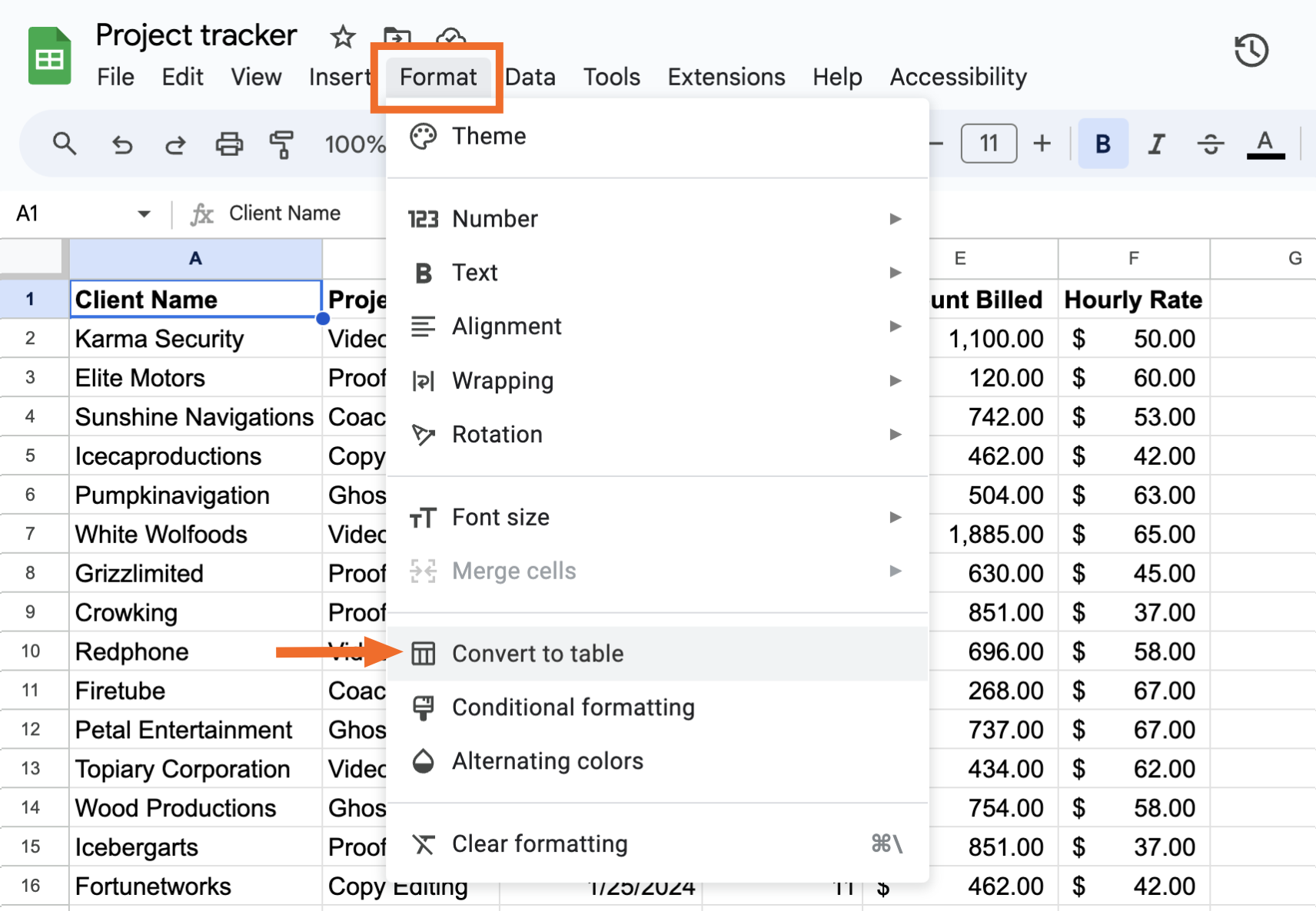
For this tutorial, I'm using a simple project management tracker filled with details like client name, project type, and amount billed.

Add column headers to the first row of your spreadsheet, if they're not already there.
Highlight the cell range containing the data that you want to turn into a table. You can also click any cell within your spreadsheet to automatically turn every column containing data into a table.
Click Format, and then select Convert to table.

Google Sheets automatically converts your data into a table, complete with distinct borders, clearly defined column headers, and the ability to sort and filter each column.

By default, Google Sheets names the table Table1. To change this, click the name and enter a more descriptive one.
To access the table menu, click the down caret (⋁) next to the table name. From here, you can do a number of things:

Adjust table range. Enter a new data range to include more or less information in your table.
Turn off alternating colors. Google Sheets automatically applies alternating colors to each row of your table, but this switches it to only one color across all rows.
Customize table colors. This option name is a little misleading—it lets you select a custom color fill for only the column headers and table name. Jump ahead to learn how to alternate row colors in Google Sheets.
Revert to unformatted data. This switches your data back into its original form.
Delete table. This deletes your data altogether.
How to make a table in Google Sheets using a template
Click Insert, and then select Tables. Or, click any cell and enter
@table.The Tables panel will appear with a whole host of pre-built table templates, grouped by category—for example, Event planning, Project management, and Travel planner. Hover over any template to get a preview.
Click the template you want to use to insert it into your spreadsheet.
Edit your table and fill in data as you normally would.

How to edit table columns in Google Sheets
Here are all the ways you can edit and manipulate table columns in Google Sheets. To access the column menu, click the down caret (⋁) next to the heading of the column you want to edit.
Edit column type. For the most part, Google Sheets will automatically treat basic data, like numbers and dates, with the appropriate formatting. But you can modify this or change it to more advanced column types, like dropdowns and checkboxes.
Sort and filter column. Use the sort and filter tools the same way you normally would.
Insert or delete a column. Add a new column within the borders of your existing table or delete the column. You can also access the same options by right-clicking a column.
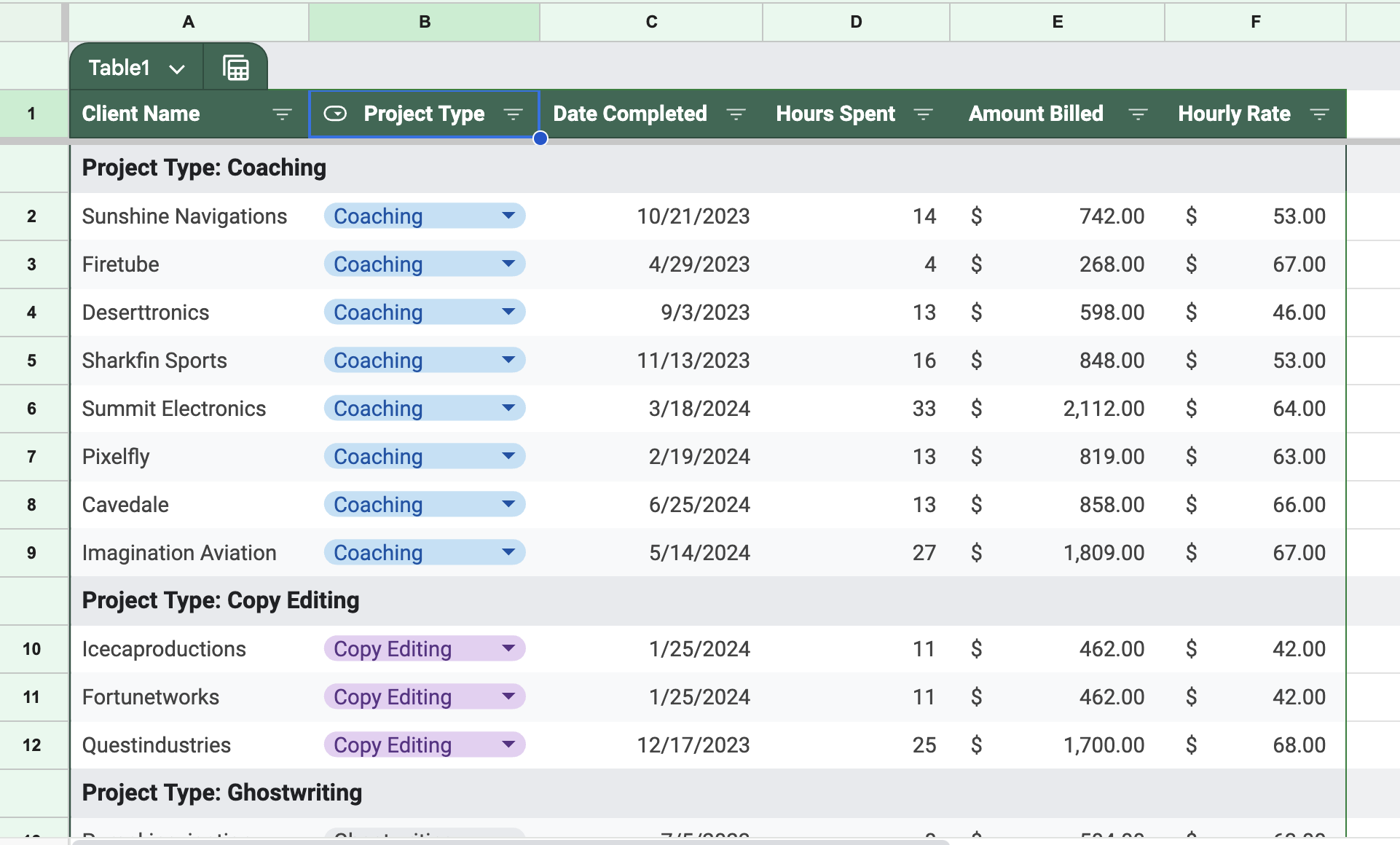
Group by column. This is a quick way to create a filter view. Google Sheets automatically groups your data based on the column. For example, if I click Group by column from the Project Type column (as shown below), it'll group all related projects together. Similarly, if I do the same thing from the Hourly Rate column, it'll group all rows billed at the same rate together.

How to alternate row colors in Google Sheets
Here's how to color every other row in Google Sheets. Note: This is an all or nothing feature—you can either alternate row colors for your whole spreadsheet or not at all.
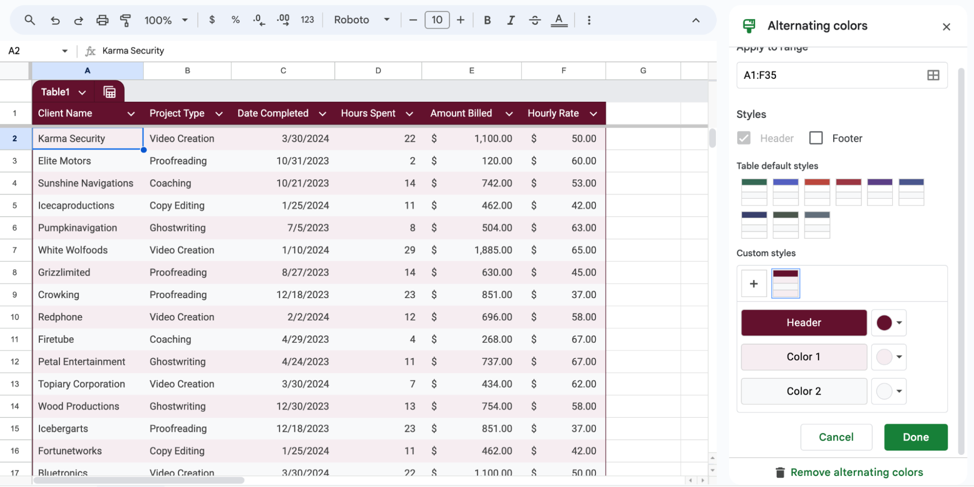
Click Format, and then select Alternating colors.
In the Alternating colors panel, change Color 1 (and optionally Color 2) in the Custom styles section. Be sure to choose a high-contrast color scheme to improve readability. For example, black text against a light pink background is easier to read than, say, a bright red background.
Click Done.

Alternatively, you can use conditional formatting to color-code your data depending on certain values. For example, you can tell Google Sheets to fill in a cell if the amount billed for a project is equal to or greater than a certain amount. This way, you're only coloring in key data.
How to manually create a table in Google Sheets in 5 steps
If you prefer to manually transform your data into a table versus applying a standard table template and editing from there, you can also do that. Here's how to manually create a table in Google Sheets.
1. Create your headers and input your data
Enter your data as you normally would. Be sure to add descriptive headers at the top of each column. Once you outline these sections and input your data, your table should look something like this.

2. Format your data
Let's say one of your columns contains dollar amounts, but the values appear as only 20.00 or 1500.00. To make it clear that these are dollar values, you'll want to change the number format to add a dollar sign ($) ahead of every value.
You can use the toolbar to quickly format your cell values, but I prefer using the Format menu.
Highlight the cell or cell range that you want to apply formatting to. In this case, that's the Value column.
Click Format > Numbers > Currency.
Google Sheets will automatically format every amount in the Value column as a dollar amount—for example,
$20.00and$1,500.00.

There are a lot of other formatting options in the Numbers menu that work for things like percentages, dates, and accounting—choose the one that makes the mose sense for your data.
3. Format your table
At this point, you'll want to outline draw the outline of your table. I like to start with the outer borders.
Highlight all the data you want to group into a table, including your column headers.
In the toolbar, click the Borders icon, which looks like a square divided into four quadrants, and then click Outer borders (or any border style you prefer).

Google Sheets will apply the border style to your selected cell range.


Now that your table is starting to take shape, you can focus on adding more flair to make your data stand out. For example, bolded headers help readers quickly pick up the format and begin reading the data.
Tweak the visual elements—like font, bolding, italics, and background color—until you find a balance you like. Here's the busy person's guide to useful tools:
Font: Access via the Font dropdown on the toolbar.
Bold and italics: Use the B and I shortcuts on the toolbar or navigate to the Format menu and then click Text.
Background color: Use the Fill color shortcut on the toolbar.
Alternating colors: Navigate to the Format menu, then click Alternating colors.
Border options: Use the Border shortcut on the toolbar.

4. Set up your filters
If you're working with hundreds of rows of data, you might find yourself scrolling endlessly to find a needle in a haystack. To save yourself time, add filters to your spreadsheet. This way, you can temporarily hide any irrelevant data, allowing you to focus on the information that matters.
Click any cell or highlight the specific columns you want to add a filter to.
Click Data, and then select Create a filter.

A filter icon will appear next to every column heading that you've applied a filter to.

5. Add rows and columns as needed
Depending on the data you're preparing, you might need to add more columns and rows to fit everything.
The easiest way to do this is to right-click a row, and click Insert 1 row above or Insert 1 row below (depending on where you want to insert it).

Do this for as many rows as you need. The function will hold on to the formatting for you, and the table will expand on its own. Input your fresh data and use your filters to reset the order.

Tips and best practices to level up your Google Sheets table game
Google Sheets provides a few more tools you can use to level up your table game. Some allow you to add a measure of automation through formulas, and others allow you to collaborate with your teammates, so no one's work clashes (in color or otherwise).
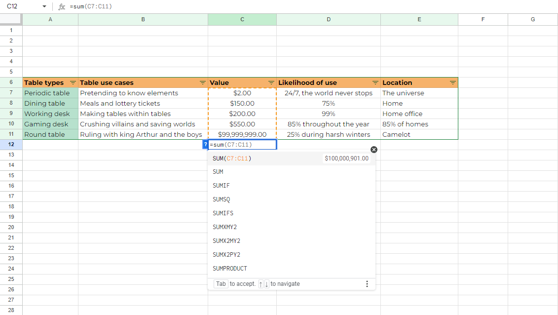
Use cell references and formulas: Google Sheets formulas can be somewhat intimidating. I, for one, sighed deeply the first time I saw the full list because I knew I likely wouldn't need or use most of them. They can be useful, though, if you want to create tables that automatically calculate values for you, such as sums. Google provides a comprehensive list of Google Sheets functions. You'll need to try a few options to find one that works for you. To add a formula, go into a cell and type an equal sign (=) followed by the function you want to use. Google Sheets will suggest formulas and ranges based on your data automatically. In the following screenshot, I added a cell that calculates the total value of my tables.
Name your tables for easy reference: I think it'll be very hard to mix up your tables, especially if you're the one who built them. But a viewer or co-editor may not have the same familiarity with the data as you do. To name your table, highlight it in its entirety, right-click it, and select Define named range. Input your table name here, and you're done. This is especially helpful if you have multiple tables in one sheet. You can use this function to quickly find tables in exceedingly complex documents. Navigate to the Data menu, and click on Named ranges to see a list of the tables you have within the sheet.

Export and import Google Sheets data: Under the File menu, you can export a Sheet by downloading it in the format you prefer (.xlsx, .ods, .pdf, .html, .csv, and .tsv).

The import feature, under the same menu, allows you to quickly add another spreadsheet's data to your work in progress. As with most Google Sheets features, it'll take a bit of testing and a lot of copy-pasting to manipulate data into taking shape. You can drag and drop CSV files, or quickly pull Sheets directly from your drive.

Collaborate with your team and use version control: If you're working on your Google Sheet with other people, you can assign them permissions to edit the document as they please. You can then use version control (File > Version history) to view every iteration of the document that's saved. This means every change anyone makes on the doc is tracked and visible, so you can revert back to an older version or zero in on a specific edit.

Utilize keyboard shortcuts for faster table creation: Personally, I like to use the toolbar at the top to navigate through my table creation. You can't rush perfection, and you shouldn't rush mediocrity, either. That said, there are a lot of keyboard shortcuts you can use (and set) to make your process smoother and faster. Here's the full list of default keyboard shortcuts.


Manage and store your data with Zapier Tables
Google Sheets is a solid option for storing and organizing your data. But if you want to get more out of your data, try Zapier Tables. It's a no-code database tool that allows you to store, edit, share, and automate your data—all in one place. It's great for lead capture and enrichment, adding approval steps to workflows, scaling an onboarding process, or anything else that requires organized data. Learn more about how to use Zapier Tables.

Zapier is the most connected AI orchestration platform—integrating with thousands of apps from partners like Google, Salesforce, and Microsoft. Use forms, data tables, and logic to build secure, automated, AI-powered systems for your business-critical workflows across your organization's technology stack. Learn more.
Related reading:
This article was originally published in April 2024 by Hachem Ramki. The most recent update was in July 2024.