Let's say you have a list of email addresses that you collected through a form on your website. You want to know how many email addresses you received, but you're worried that someone may have filled out the form twice, which would inflate your numbers.
When you're working with large amounts of data in a spreadsheet, you're bound to have duplicate records. Whether it was human error or robots that put them there, those duplicates can mess with your workflows, documentation, and data analysis.
Here, I'll show you how to find duplicates in Google Sheets, so you can decide whether or not to delete them yourself. I'll also walk through how to automatically remove duplicates and create a list of unique values.
Table of contents:
How to find duplicates in Google Sheets
The easiest way to find data doppelgängers is to highlight all duplicate content using conditional formatting and a custom formula. What's the formula? It doesn't matter because now that Gemini is integrated into Google Sheets, you can simply ask Gemini to find and highlight duplicates for you. (But if you want to feel like you've really earned your Spreadsheet Savant badge on LinkedIn, jump ahead for the manual steps.)
Click any cell in your spreadsheet.
Enter the equal sign (
=), and select Generate formula with Gemini.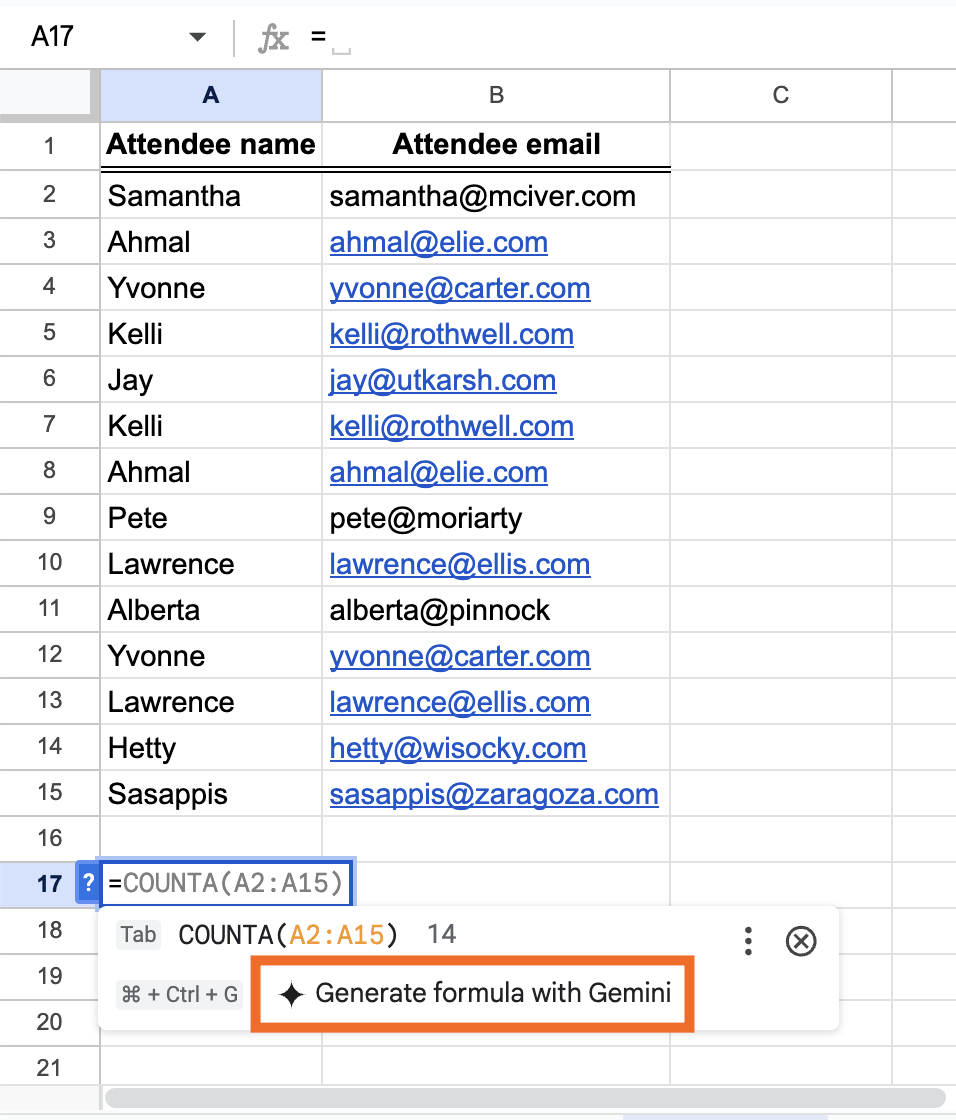
In the Gemini chat, tell the AI what you want it to do. For example: "Create a formula that finds and highlights every duplicate value in light orange."
Press Enter.
Gemini will respond with a suggested plan and formula.
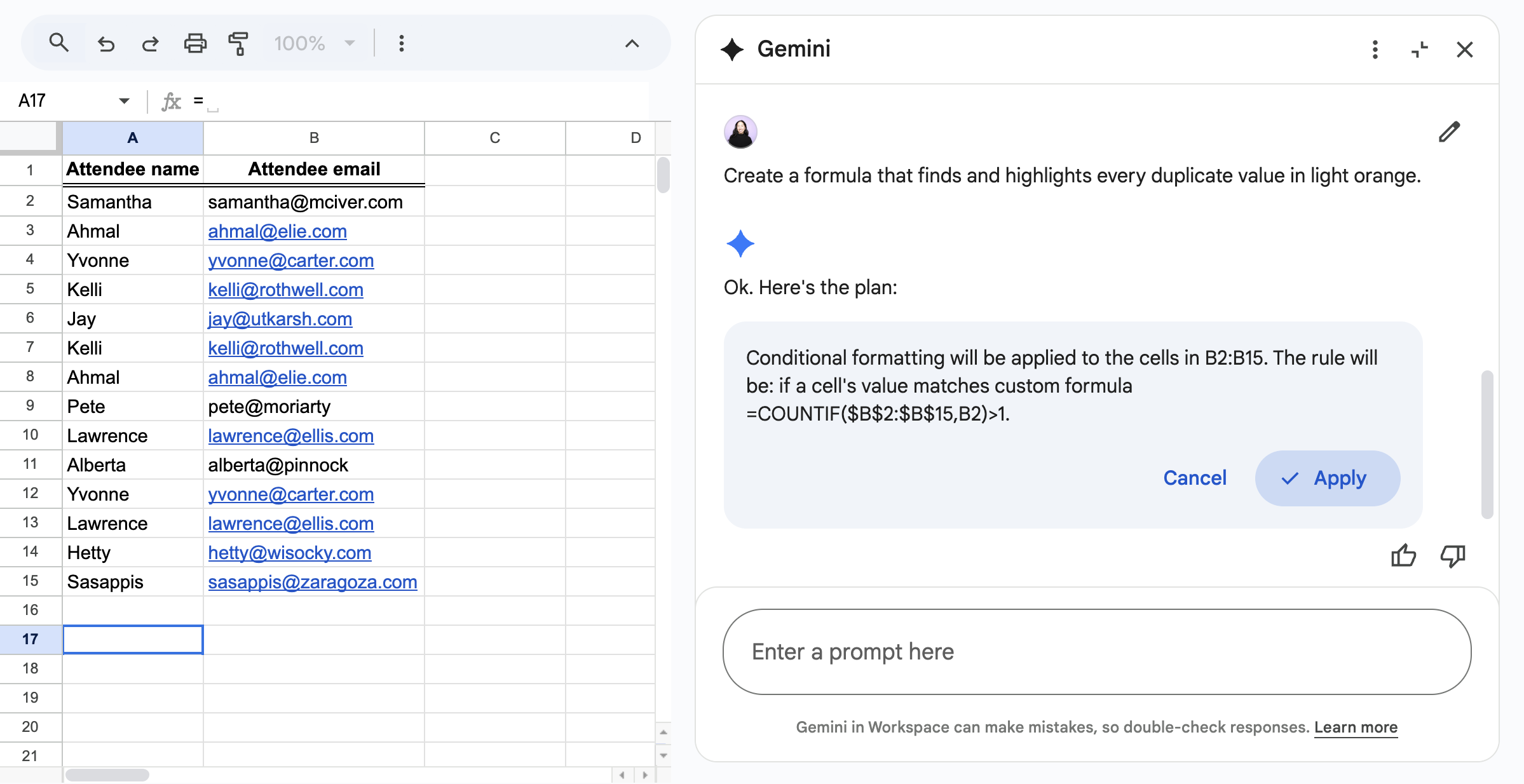
Click Apply.
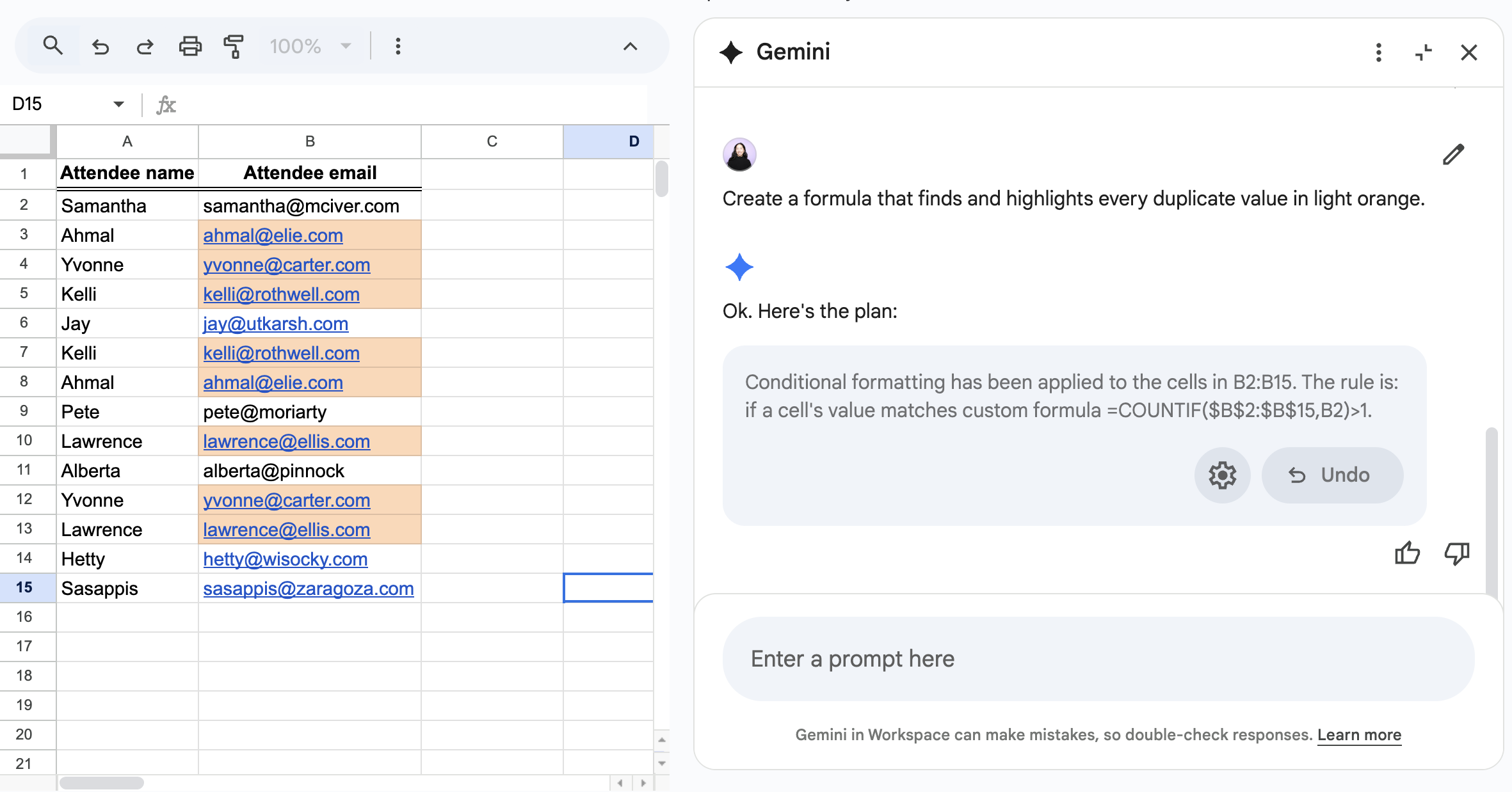


That's it.
How to manually highlight duplicates in a single column in Google Sheets
If you get a kick out of manually setting conditional formatting rules, here's how to set up a rule to help you spot repeat values in a single column.
Highlight the data range you want to check for duplicate information. Then select Format > Conditional Formatting.
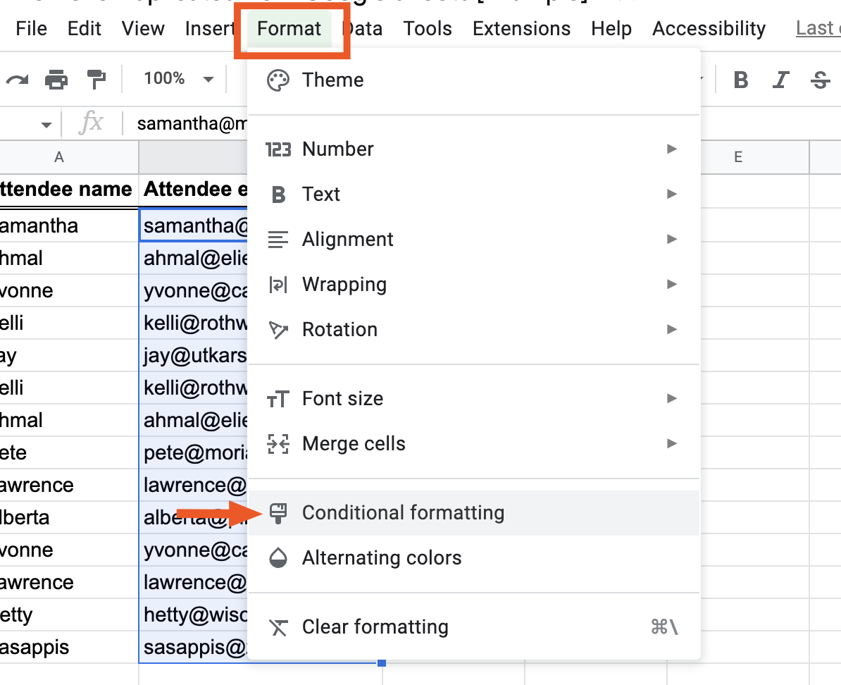
From the Conditional format rules window that appears, click the dropdown menu under Format rules, and select Custom formula is.
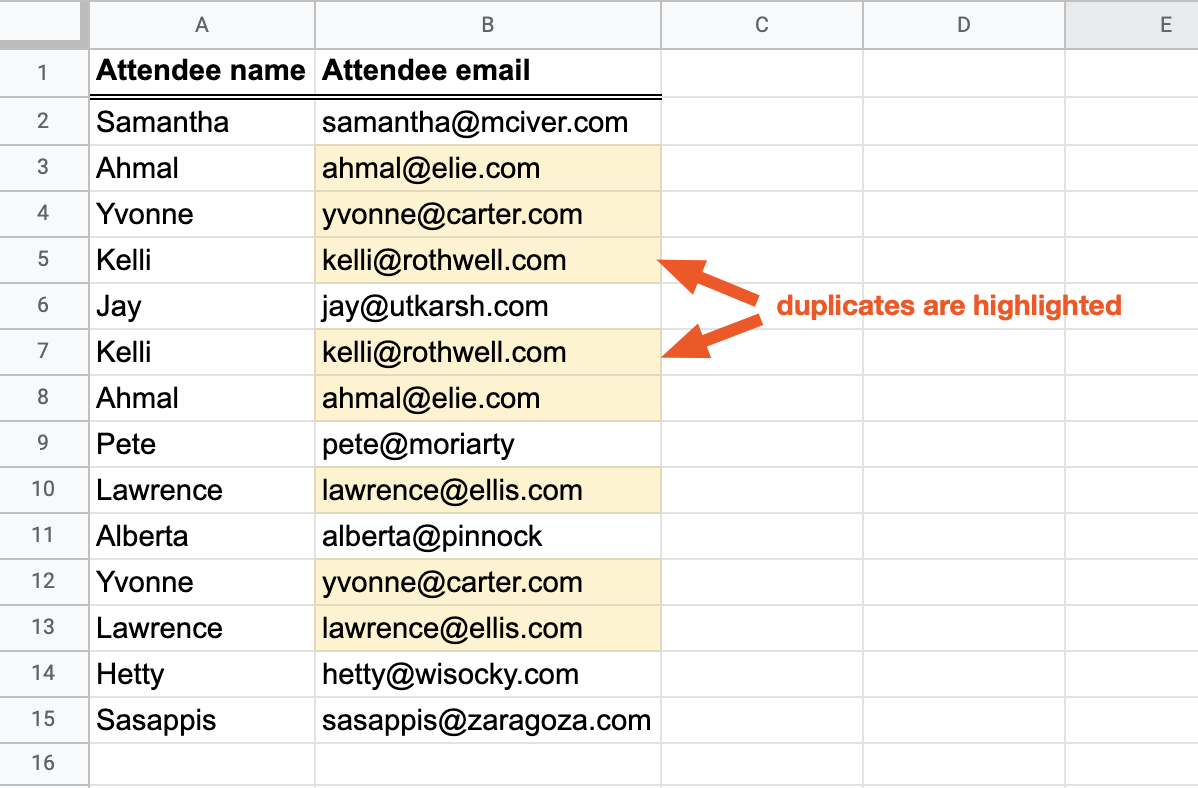
Enter a custom duplicate checking formula in the Value or formula bar. In this example, we're looking for duplicates in cells B2:B15, so the custom formula is
=COUNTIF($B$2:$B$15,B2)>1. If your duplicates are in a different data range (for example, A2:A15), your custom formula would be=COUNTIF($A$2:$A$15,A2)>1.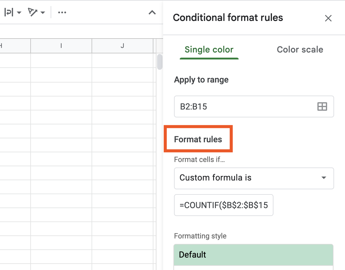
Customize how your duplicates will appear on the spreadsheet under Formatting style. By default, Google Sheets will highlight duplicate data in green. Then click Done. (Tip: If you change the fill color, choose a high-contrast color scheme, such as light yellow 3, to improve readability.)

You can now review the duplicate data (highlighted) and decide whether you need to delete any redundant information.


How to highlight duplicates in multiple rows or columns in Google Sheets
If you have duplicate data in multiple rows or columns, repeat steps one to three from above, but change the custom duplicate checking formula to =COUNTIF($A:$Z,Indirect(Address(Row(),Column(),)))>1.
Tip: If you only want to scan for duplicates in specific rows or columns, simply update the data range under Apply range to match the cell range you want to check for repeats.

Customize how your duplicates will appear on the spreadsheet under Formatting style. Then click Done.

How to remove duplicates in Google Sheets
If you want to dive right into nixing redundant data without manually reviewing them first, Google has made this really easy to do. It's not as simple as telling a chatbot to make duplicates disappear, but the feature is accompanied by a sparkly wand, so it's just as fun. Here's how to remove duplicate data in Google Sheets.
Click any cell that contains data. Then, select the Data tab > Data cleanup > Remove duplicates.

From the Remove duplicates window that appears, select which columns you'd like to include in your search for duplicate data. Click Remove duplicates.
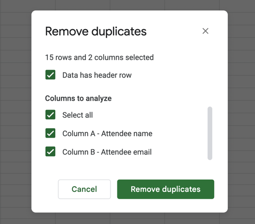
Note: If your spreadsheet includes a header row, be sure to select Data has header row, so that Google Sheets ignores this row when removing duplicates.
Google Sheets will let you know how many duplicate values were removed.


Bonus: How to find unique values in Google Sheets
If you want to keep your original data and get a list of unique values (data that's not duplicated) from a data range, the simplest way is to ask Gemini to do this. Enter this prompt: "Give me a list of only unique values."
Behind the scenes, Gemini will run a UNIQUE function, and then return a list of unique values, which you can then insert or copy and paste into your sheet. Note: If you insert Gemini's output, it'll overwrite your existing data.

Automate Google Sheets with Zapier
If you're going through the effort of manually finding and cleaning up duplicates in Google Sheets, chances are you're also juggling other repetitive spreadsheet tasks. Use Zapier's Google Sheets integration to automate those workflows instead. Zapier lets you connect thousands of apps together so you can orchestrate multi-step, AI-powered workflows that scale across teams and systems.
For example, you can set up a workflow that takes new form entries, uses AI to check for duplicates before they ever land in your sheet, enriches the valid ones with extra context, and then routes high-value leads to your CRM. Instead of constantly tidying up, you’re building a system that keeps data clean and useful from the start.
Discover more ways to automate Google Sheets, or get started with one of these pre-made templates.
Save new Gmail emails matching certain traits to a Google Spreadsheet
Create Google Sheets rows for new Google Ads leads
Send emails via Gmail when Google Sheets rows are updated
Zapier is the most connected AI orchestration platform—integrating with thousands of apps from partners like Google, Salesforce, and Microsoft. Use forms, data tables, and logic to build secure, automated, AI-powered systems for your business-critical workflows across your organization's technology stack. Learn more.
Related reading:
This article was originally published in May 2018 by Deb Tennen. The most recent update was in September 2025.