Whenever I'm working with large datasets in Google Sheets, it's easy for me to lose track of what's what—especially without headers locked in place. Take this simple student grade sheet below, for example.
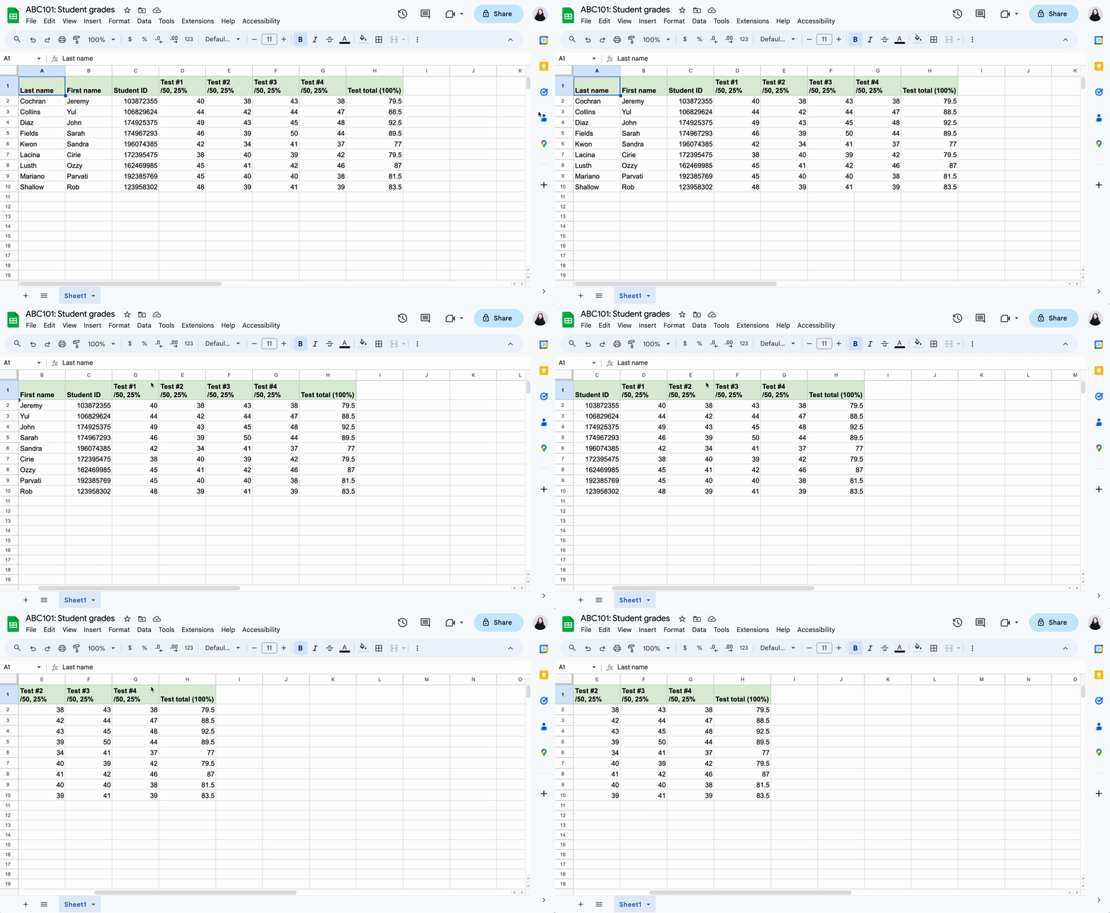
Notice that as I scroll across the sheet, the student names and IDs disappear. With this view, it's nearly impossible for me to remember which grade belongs to which student.
That's where the Freeze function comes in. It lets you pin columns in place so you can see the data you need at all times, even as you scroll through your spreadsheet.
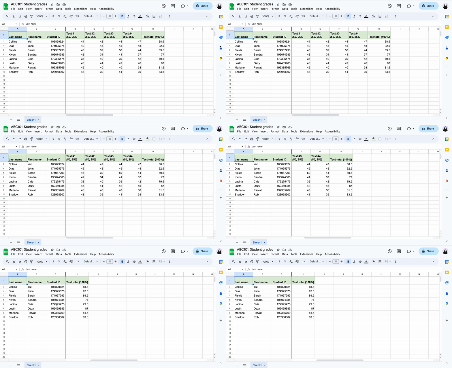
How to freeze columns in Google Sheets
Here's the easiest way to freeze a column or multiple columns in Google Sheets.
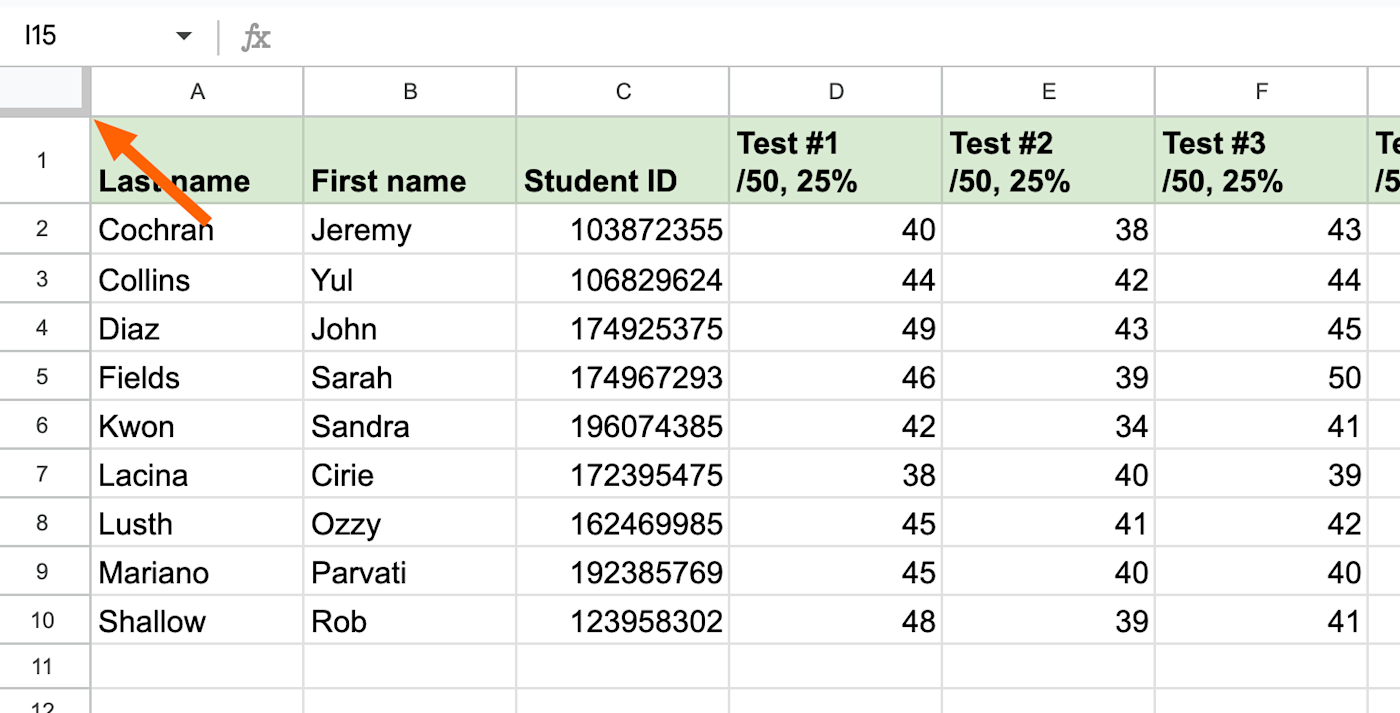
In the top-left corner of your spreadsheet, next to column A and above row 1, there are two thick, gray bars running horizontally and vertically.
To freeze a column, click the vertical bar and drag it across to the right side of the last column you want to freeze. For example, let's pin up to the student IDs in column C.
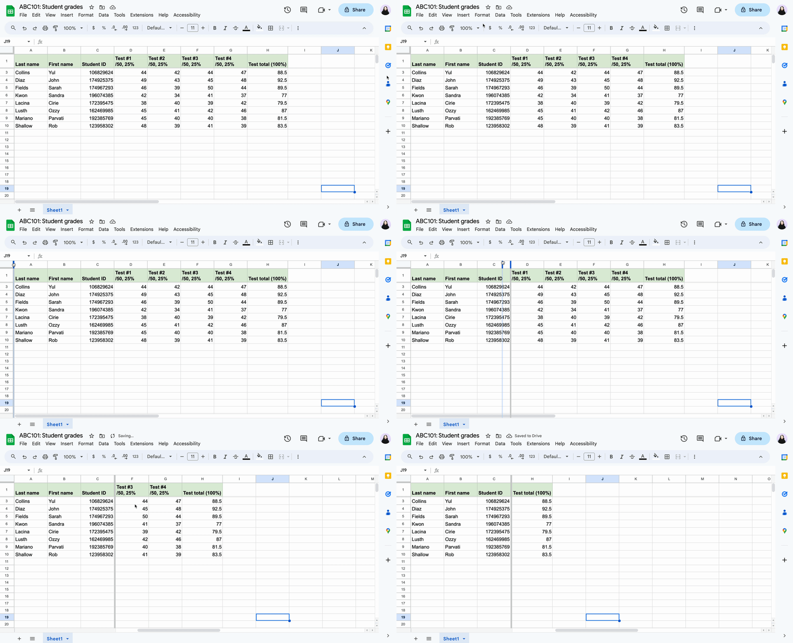
To unfreeze a column, drag the bar back to its original position.
If you, like me, get frustrated about having to get your cursor in just the right spot, there's another way.
Open a Google Sheets spreadsheet.
Select the columns you want to freeze.
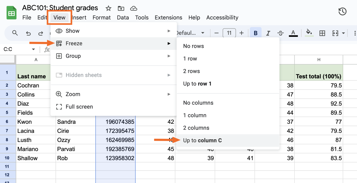
Click View, and then select Freeze.
Click Up to column [column letter].
Let's freeze the student IDs in column C again using this method. For this example, click View, select Freeze, and select Up to column C.
It's a simple example, but when you're reviewing grades for 30 or so students—or you're working with a large dataset of any sort—freezing columns and rows makes scrolling through the data much more manageable.
To unfreeze a column, repeat the same steps, but instead of clicking Up to column C, click No columns.
Automate Google Sheets
Manual data entry is ripe for human error. With Zapier, you can connect Google Sheets with your go-to apps. This way, you can automate your most time-consuming spreadsheet-related tasks. For example, you can automatically add new lead data and form submissions to an existing spreadsheet. Learn more about how to automate Google Sheets, or get started with one of these workflow templates.
Collect new Typeform responses as rows on Google Sheets
Add Google Sheets rows for new Google Forms responses
Add new Facebook Lead Ads leads to rows on Google Sheets
Add new leads in LinkedIn Ads to Google Sheets rows
To get started with a Zap template—what we call our pre-made workflows—just click on the button. It only takes a few minutes to set up. You can read more about setting up Zaps here.
Related reading:


