We independently review and test every app we write about. When you click some of the links on this page, we may earn a commission. Learn more.
You can use Google Sheets to do practically anything. There's the serious stuff, like organizing to-do lists, managing leads, and making decisions. And then there's the fun stuff, like playing Wordle, simulating a baseball game, and making custom browser homepages.
But before you can make a spreadsheet to track the number of minutes your dog has gone by without being told he's a good boy—or the stuff that helps you get actual work done—you have to understand the basics.
In this Google Sheets tutorial for beginners, I'll walk you through everything you need to know about how to use Google Sheets.
Table of contents:
What is Google Sheets?
Google Sheets is a spreadsheet app used to organize, format, and calculate data. It's included as part of Google Workspace—a suite of connected productivity tools, including Google Docs, Google Forms, and Google Slides.
You can access Google Sheets via the web, its mobile app (available for Android and iOS), and desktop app (available only on Google's ChromeOS).
Is Google Sheets the same as Excel?
Google Sheets and Excel are both spreadsheet apps, so there are a lot of overlapping features. But there are a few key differences.
Collaboration. Google Sheets was designed with collaboration in mind—that's why it's so easy to share worksheets with various permission settings. Excel has similar collaboration features—for example, you can add and edit comments—but the experience isn't as smooth as what you get with Google Sheets.
Cell limits. Google Sheets has a cell limit of 10 million, but that pales in comparison to Excel's 17 billion cells per spreadsheet. That's what makes Excel the better tool for dealing with big data.
Formulas. Excel has more powerful formulas and data analysis features, including built-in statistical analysis tools and extensive data visualization options. Google Sheets, on the other hand, offers a "lite" version of most of these features—but they're nowhere near as in-depth.

For a detailed breakdown of how these two apps stack up, check out our app showdown: Google Sheets vs. Excel.
Google Sheets basic terms
To kick things off, let's cover some spreadsheet terminology you'll need to know when using Google Sheets:
Cell: A single data point or element in a spreadsheet.
Column: A vertical set of cells.
Row: A horizontal set of cells.
Range: A selection of cells extending across a row, column, or both.
Function: A built-in operation from the spreadsheet app you'll use to calculate cell, row, column, or range values and manipulate data.
Formula: The combination of functions, cells, rows, columns, and ranges used to obtain a specific result.
Worksheet (Sheet): The named sets of rows and columns that make up your spreadsheet. One spreadsheet can have multiple sheets.
Spreadsheet: The entire document containing your worksheets.
How to create a spreadsheet in Google Sheets
There are four ways to create a new spreadsheet in Google Sheets.
From the Google Sheets dashboard
Go to docs.google.com/spreadsheets.
Click Blank spreadsheet.

From an existing Google Sheets spreadsheet
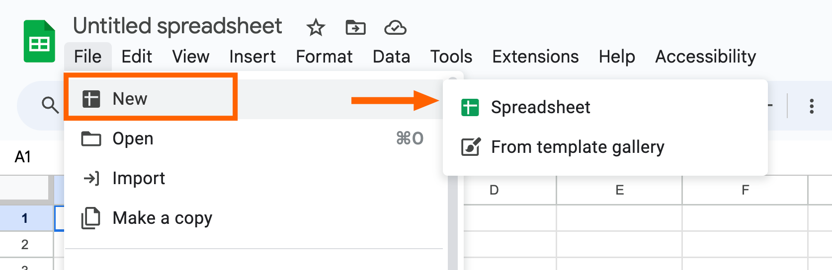
With Google Sheets open, click File.
Click New.
Click Spreadsheet to create a blank spreadsheet or From template gallery to use a template.

Google Sheets offers a limited set of pre-built spreadsheet templates. To expand your options, check out these free Google Sheets templates.
From Google Drive
Go to drive.google.com.
In the side menu, click New, and then select Google Sheets.
Select Blank spreadsheet or From a template.

From your browser's address bar
With your browser open, enter sheets.new into the address bar.
Press Enter.
A new tab with a blank Google Sheet will appear in your browser window.

How to add data in Google Sheets
When you create a new spreadsheet, you can immediately begin typing, and your data will automatically appear in the top-left cell. If you want to enter data somewhere else, click another cell and type away. A blue border will appear around the cell you're typing in to make it easier to identify which cell you're working with.

To make it easier to filter or manipulate data later on, each cell should contain only one value—for example, 100 or Mango.
When you finish entering data into a cell, you can do one of four things:
Press Enter or return to save the data and move to the beginning of the next row.
Press Tab to save the data and move one cell to the right in the same row.
Use your arrow keys (up, down, left, and right) to move one cell in that direction.
Click any cell to jump directly to it.
If you don't want to type in everything manually, you can also import data into Google Sheets en masse using a few different methods:
Copy and paste a list of text or numbers into your spreadsheet.
Copy and paste an HTML table from a website.
Import an existing spreadsheet. If you're importing data from another Google Sheet, you can also use the IMPORTRANGE function to automatically pull in that data and keep things consistent.
Use the fill handle to automatically populate neighboring cells with data.
How to import data to Google Sheets
If you want to pull in data from an existing spreadsheet, you'll first have to export that spreadsheet's data into an acceptable file format—for example, .csv, .xls, or .xlsx.
With Google Sheets open, click File > Import.
Choose the file you want to import. You can upload a file directly from Google Drive or your computer.
Click Insert.
In the Import file popup, you can modify the following:
Import location. This gives you a handful of ways to import your data. For example, you can import your data into your current sheet, add it as a new sheet, or create a new spreadsheet altogether.
Separator tab. Google Sheets will automatically detect and apply this, but you can also choose a specific type: Tab, Comma, or Custom.
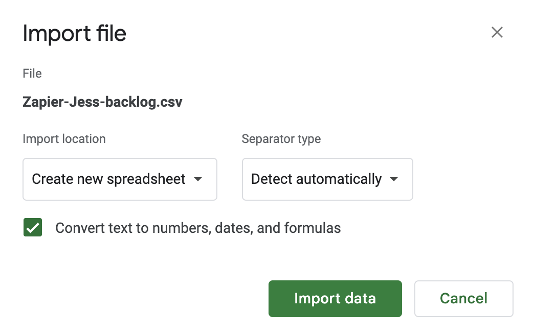
Click Import data.

How to use the fill handle in Google Sheets
The fill handle in Google Sheets offers a convenient way to populate data or copy formulas and data in adjacent cells. Hover your cursor over the bottom-right corner of any cell or cell range, and it'll automatically turn into the fill handle—it looks like a plus sign (+).

By dragging the fill handle across or down a range of cells, you can perform a number of tasks:
Copy a cell's data, including any formatting, to neighboring cells.
Copy a cell's formula to neighboring cells.
Create an ordered list of data.
The value Google Sheets populates in the neighboring cells will vary depending on the type of data contained in the original cell or cell range that the fill handle originated from.
For example, if you select only one cell, the value of the selected cell will appear in every cell that you drag the handle over.

If you select a series of neighboring cells, Google Sheets will repeat the pattern across or down the cells that you drag the handle over. In the example below, I've selected three neighboring cells, each containing a unique value: Mango, Coconut, and Pineapple. When I drag the fill handle, the pattern repeats across the row so that it's Mango, Coconut, Pineapple, Mango, Coconut, Pineapple, and so on.

If you want to use the fill handle to create an ordered list, highlight at least two cells containing the sequence you want Google Sheets to continue, and then drag the fill handle.

When it comes to ordered lists, there's one caveat worth mentioning.
Unlike copying text values to neighboring cells, Google Sheets will only continue sequences for number values—not repeat them. For example, if I wanted to repeat the pattern Employee 1, Employee 2, Employee 3 across the row, Google Sheets wouldn't be able to. It would just keep counting up. I would have to manually copy and paste the values across instead.
To make things confusing, if I select a cell range containing an arbitrary set of numbers—for example, Employee 1, Employee 17, and Employee 20—Google Sheets would repeat this pattern since there's no logical sequence to continue.
How to automatically import data using Zapier
Don't want to spend precious time manually importing data into Google Sheets? Automate the process instead. With Zapier's Google Sheets integration, you can automatically pull data from other apps into your spreadsheet and orchestrate multi-step, AI-powered workflows. For example, you can import customer feedback from an online form, use AI to categorize those responses into specific segments or topics, and flag feedback that meets certain criteria for personalized follow-up.
Learn more about how to automatically add data to Google Sheets, or get started with one of these pre-made templates.
Add Google Sheets rows for new Google Forms responses
Create Google Sheets rows for new Google Ads leads
Add new Facebook Lead Ads leads to rows on Google Sheets
Zapier is the most connected AI orchestration platform—integrating with thousands of apps from partners like Google, Salesforce, and Microsoft. Use forms, data tables, and logic to build secure, automated, AI-powered systems for your business-critical workflows across your organization's technology stack. Learn more.
How to use the Google Sheets toolbar
The Google Sheets toolbar is where you'll find all your basic tools and formatting options. Depending on the width of your screen, some of the tools may be hidden. To reveal them, click the More icon, which looks like three dots stacked vertically (⋮).

Hover over any icon to discover its function. Or click on it to expand that tool's options, if applicable. Tools like Borders, Comments, and Align work similarly to what you'd expect from Google Docs.
If you can't find a tool or want to check if a tool exists, the quickest way to find out is by using the search tool. Click the Search the menus icon, which looks like a magnifying glass.
Unlike how you can hide the toolbar in Excel, Google Sheets gives you the opposite ability: you can hide everything above the toolbar, including the spreadsheet name and tabs, allowing you to focus on the spreadsheet itself. To do this, click the up caret (⋀) in the toolbar or use your keyboard shortcut: Ctrl+Shift+F (on Mac and Windows). Click the caret or enter the keyboard shortcut again to make everything reappear.

Now back to using the Google Sheets toolbar.
The best way to show you how to use some of the most common Google Sheets formatting tools is to work through an example. Let's edit this simple project tracker.

How to format data in Google Sheets
To start, let's make the headers in the first row stand out.
Click the cells you want to format. To apply the same formatting to neighboring cells, select the first cell, and drag your cursor across or down the cell range. To apply the same formatting to cells that aren't connected, select one cell, press and hold
commandon a Mac orCtrlon Windows, and then select the other cells. Your cell selection will remain selected unless you click on a different cell, which is convenient if you want to edit multiple formatting options.From the toolbar, click the plus sign (
+) next to the font size to increase it to 12. Or you can enter 12 in the Font size field.Click the Bold icon, which looks like the letter
B.Click the Fill color icon, which looks like a paint can, and select a theme color. I'm using a light shade of green.
Click the Align icon, which looks like a stack of horizontal lines. By default, it's set to Horizontal Align. Click Center.

The headings are more obvious now. But some of the heading names are cut off. Let's fix that.
How to make Google Sheets cells expand to fit text
There's a default setting in Google Sheets called Overflow that allows cells with long strings of text or numbers to bleed into the neighboring cell. But once you enter data into that neighboring cell, that long string of text will get cut off.
The easiest way to expand the cell to fit your text is by double-clicking the border on the right side of the column you want to expand. Google Sheets will then expand it to fit the longest value in that column.

You can also expand the width of multiple columns at once.
Highlight the columns you want to resize.
Right-click your selection.
Click Resize columns [names of columns selected].
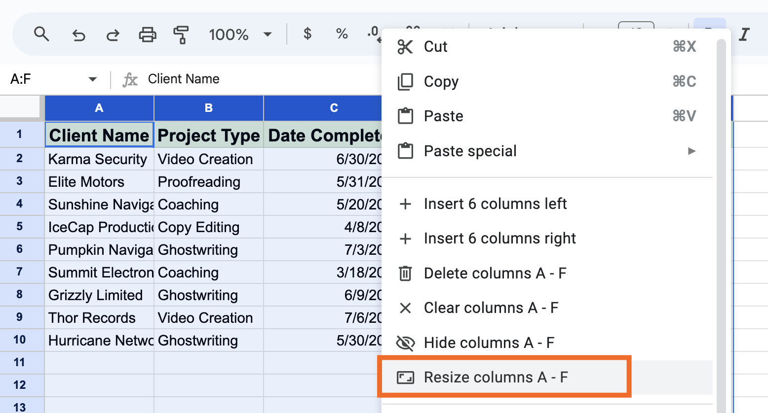
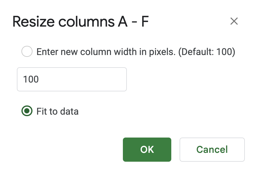
In the Resize columns popup, click Fit to data.
Click OK.


That's it. No more smooshed data.

How to wrap text in Google Sheets
Let's say you want to leave your columns a set width. There's another way to make sure each cell's data is still visible within a too-small column: wrap the text.
Click the cell or cells you want to apply the text wrap to.
Click the Text wrapping icon in the toolbar, and then select the Wrap icon.
Google Sheets will automatically change the row height to fit the data.

For a step-by-step guide, check out how to wrap text in Google Sheets.
How to freeze columns and rows in Google Sheets
If I scroll down through the project tracker, the column headers will quickly disappear from view. To lock the headers in place, let's freeze the first row. Here's the easiest way to do this.
In the top-left corner of your spreadsheet, next to column A and above row 1, find the thick gray bar running horizontally.
Click and drag the bar under the last row you want to freeze. In this case, that's row 1.

To unfreeze the row, drag the bar back to its original position.
You can also use the same method to freeze columns in Google Sheets—just drag the vertical bar instead.
For another option that doesn't require you to place your cursor in just the right spot, check out our article on how to freeze columns and rows in Google Sheets.
How to hide columns and rows in Google Sheets
When you're working with endless rows of data, it's easy to lose track of what's what. One way to help you focus is by temporarily hiding any rows of irrelevant data.
Highlight the rows or columns you want to hide.
Right-click your selection.
Click Hide rows [numbers of rows selected].

You'll know rows are hidden if there are numbers missing from your row headers. Or, in the case of columns, missing column letters.
To make the rows visible again, click the arrows that appear in lieu of the hidden rows.

For a step-by-step guide, check out how to hide rows in Google Sheets.
How to add a sheet in Google Sheets
You can add another sheet to your existing spreadsheet using one of two methods: add a new blank sheet or duplicate and existing one. Here's how to do both.
How to add a new blank sheet
If you want to add a blank sheet to your existing spreadsheet, click the Add sheet icon, which looks like a plus sign (+), at the bottom of your existing spreadsheet.

How to duplicate a Google Sheet
You can also make a copy of a sheet in Google Sheets.
Click the down caret (
⋁) next to the tab with the name of the sheet you want to duplicate.Click Duplicate.
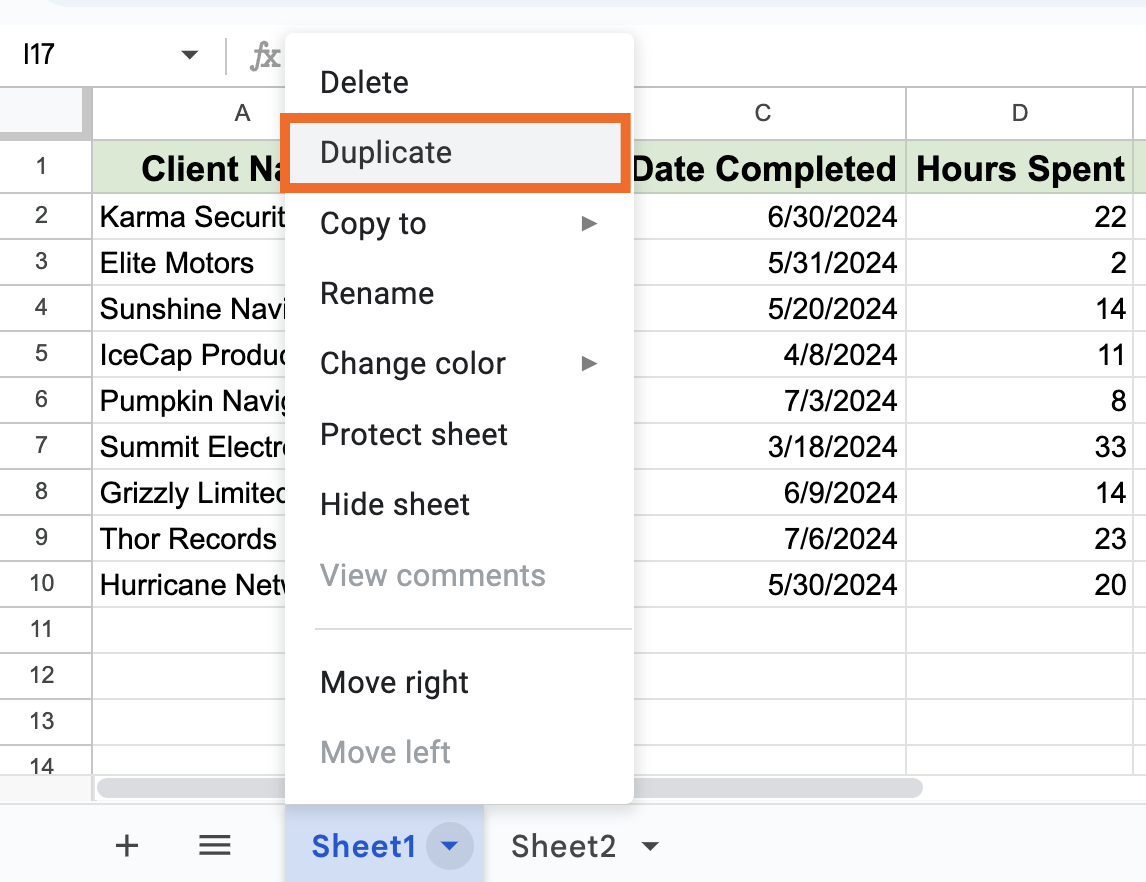
Double-click the sheet's tab to rename it.

How to use Google Sheets formulas
Like most spreadsheet apps, Google Sheets offers a bunch of built-in formulas to help you process a number of statistical and data manipulation tasks. You can also combine formulas to create more powerful calculations and string tasks together. If you're already accustomed to crunching numbers in Excel, most of the formulas work in Google Sheets the exact same way.
As a refresher, a function is a predesigned formula that's built into the app, whereas a Google Sheets formula is any equation you come up with. Before you spend time creating new formulas, it's helpful to understand which functions are already available.
Here's a quick overview of the most common basic Google Sheets functions.
SUM: adds all the values in a cell range. For example,
=SUM(D2:D10)in our spreadsheet would add up all the hours spent across cells D2 to D10.AVERAGE: returns the average of a range of cells. For example,
=AVERAGE(D2:D10)would return 16.COUNT: counts the number of cells in a given range that contain numbers. For example,
=COUNT(D2:D10)would return 9 because every cell in that range contains a number. If I deleted the value in cell D5, the count would automatically change to 8.MAX: returns the highest value in a cell range. For example
=MAX(D2:D10)would return 33.MIN: returns the lowest value in a cell range. For example,
=MAX(D2:D10)would return 2.
You can also browse through Google Sheets's extensive library of functions for a complete breakdown.
How to use Google Sheets functions
There are two main ways to use a Google Sheets function.
Enter the function name in the cell
One way to insert a function in a cell is to enter the equal sign (=) immediately followed by the function name. Google Sheets will autocomplete the function name and suggest what data you should include in the function. For example, when I enter =SUM in cell E12, Google Sheets finishes the formula by suggesting =SUM(E2:10). Google Sheets will also suggest a list of other related functions. To accept the suggested formula, press Tab.

Another option: After you enter =, click Generate formula with Gemini in the dropdown. From there, you can ask Gemini to create a formula for you using plain English—for example, "Tell me which project generates the most amount billed, on average."
Learn more about how to use Gemini.
Choose from the Function menu
Click the cell you want to enter the function into.
Click Insert, and then select Function.
Click the function you want to use.
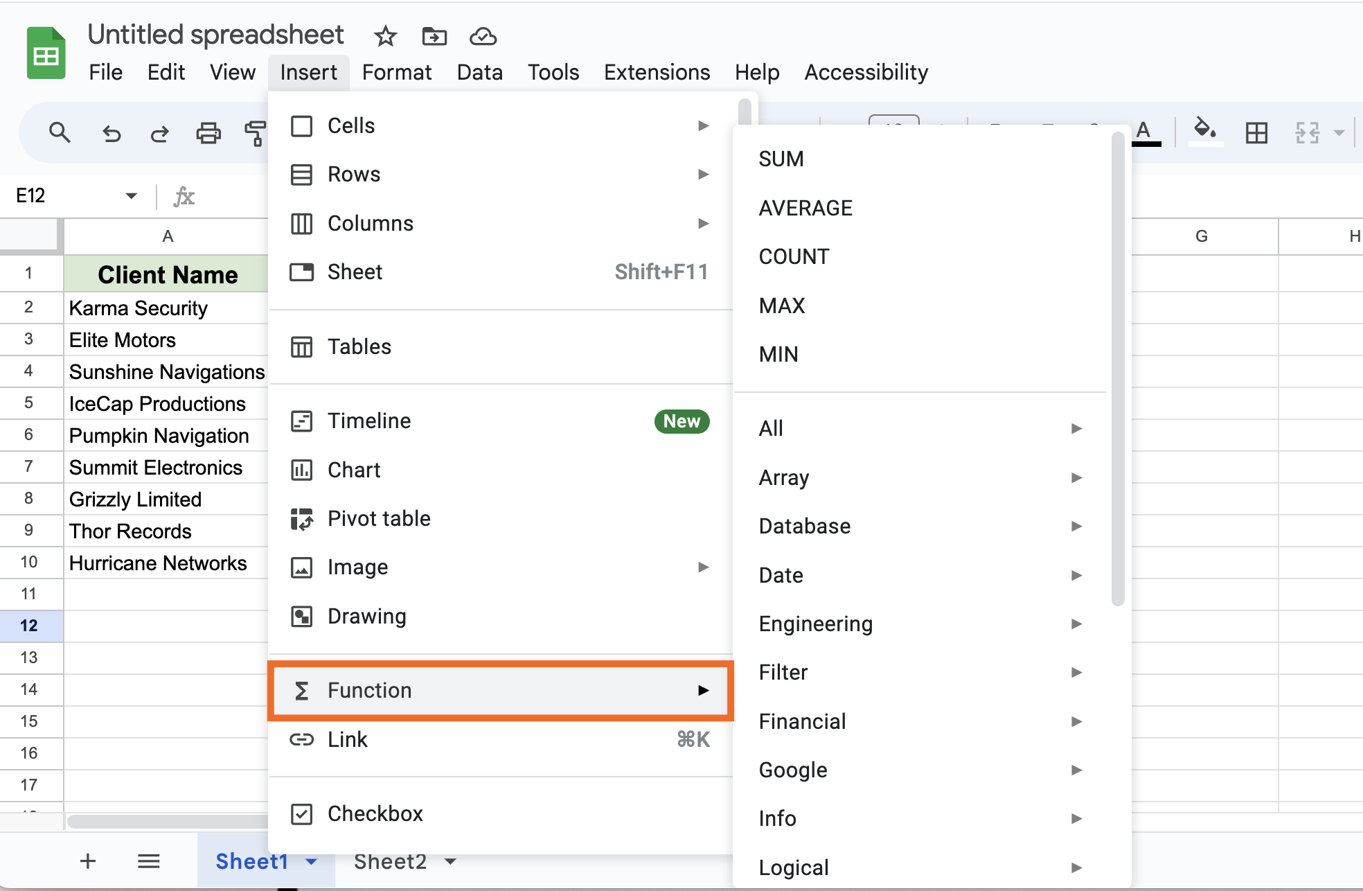
Google Sheets will populate the function in your cell, along with the parentheses where you'll need to enter your argument—the information you want the formula to calculate. For example, in the formula
=SUM(E2:E10), the argumentE2:E10tells Google Sheets to add the values of cells E2 to E10.

Now let's get back to how to use Google Sheets formulas.
To create a formula to calculate simple arithmetics, like adding, subtracting, or multiplying, you need to use specific symbols.
To add: use the
+sign.To subtract: use the
-sign.To multiply: use the
*sign.To divide: use the
/sign.To use exponents: use the
^sign.
Remember: Every formula must begin with an equal sign (=) immediately followed by the formula. By default, Google Sheets will use PEMDAS to determine the order of operations (what to calculate and in what order): Parentheses first, followed by Exponents, Multiplication, Division, Addition, and then, finally, Subtraction.
For example, if I enter =10-5*2, Google Sheets will return 0. But if I enter =(10-5)*2, it'll return 10.
If you have a series of calculations that need to happen in a specific order, use PEMDAS.
How to create a pivot table or chart in Google Sheets
Now that you know how to create a spreadsheet, import data, and use formulas, let's go over more advanced ways to manipulate and visualize your data.
How to create a pivot table in Google Sheets
A pivot table is a helpful way to analyze large data sets. With a pivot table, you can use the same data, manipulate it however you want, and get new insights each time—you don't have to create a new spreadsheet for each analysis.
We have an in-depth tutorial on how to create and use pivot tables in Google Sheets, but here's a quick overview.
Select all of the cells with the source data that you want to use, including column headers.
Click Insert, and select Pivot table.
Choose if you want to insert your table into a new sheet or an existing one.
In the pivot table editor, add the rows and columns you want to analyze, along with the values you want to display within each row and column.

The data in your pivot table will automatically change if the source data changes. If you don't see the changes reflected in your pivot table, refresh your page. It may take a minute to update, depending on the volume of data changes.
How to create a chart in Google Sheets
Let's say I want to quickly visualize how much time each client spent on their project. One way to do this would be to create a chart.
Select all of the cells with the source data you want to use, including column headers.
Click Insert, and then select Chart.
By default, Google Sheets will turn your data into a bar graph, and, for some odd reason, it'll place that graph directly on top of your source data. To modify the chart or to use a different type altogether, use the Chart editor. Alternatively, you can tell Gemini (the prompt bar's at the top of the side panel) what kind of chart you want to create, and it'll take care of the rest.
Click any of the blue dots surrounding the border of your chart to resize it. You can also drag and drop the chart to reposition it.

If you want to make more edits later on, right-click the chart and select the field you want to edit. Clicking any field will bring the full Chart editor back into view.
How to share and collaborate in Google Sheets
There are a few ways to share your spreadsheet, but here's the easiest one:
Click Share above your spreadsheet.
In the Share popup, you can:
Enter the names or email addresses of people you want to share the spreadsheet with.
Click Copy link to share a link to your spreadsheet.
Any individual you give spreadsheet access to will automatically have full Editor permissions—they can make changes, leave comments, and give others access to the file. To change this, click Editor next to their name and choose their permission level: Viewer or Commenter. You can also set an access expiration date from here.
Click Save.

In addition to sharing with specific people, you can also give general access to anyone in your organization or anyone with the link.
Word of advice: If your spreadsheet contains cell ranges that shouldn't be tampered with, lock cells in Google Sheets before sharing it.
Automate Google Sheets with Zapier
Google Sheets is often the backbone of how teams store and organize data, but the real value comes when you use that data to power the rest of your business's workflows. Wen you use Zapier's Google Sheets integration, you can orchestrate multi-step, AI-powered workflows that turn a static spreadsheet into part of a larger system.
For example, every new online order on your eCommerce site can be automatically logged in Google Sheets, then passed through ChatGPT to generate a personalized thank-you note, enriched with CRM data to include loyalty status, and then routed through your email platform for delivery.
Discover more ways to automate Google Sheets, or get started with one of these pre-made templates.
Save new Gmail emails matching certain traits to a Google Spreadsheet
Create Google Sheets rows for new Google Ads leads
Send emails via Gmail when Google Sheets rows are updated
Related reading:
This article was originally published in July 2016 with contributions from Michael Grubbs and Shea Stevens. The most recent update was in September 2025.