I'm the kind of human who, when presented with too much information, short circuits. It's the case with restaurant menus that read more like textbooks (looking at you, Cheesecake Factory). And it's the same thing with Google Sheets.
One way for me to reduce information overload while parsing data is to make unnecessary information temporarily disappear.
Here, I'll show you how to hide rows in Google Sheets. (The same thing works to hide columns, too.)
It's worth noting, though, that hidden rows and columns will still be included in any formulas used in your spreadsheet. If you plan on using formulas, I recommend using filters to first narrow down your data instead.
How to hide rows in Google Sheets
Here's the easiest way to hide rows in Google Sheets.
Open a Google Sheets spreadsheet.
Select the rows you want to hide.
Right-click your selection, and click Hide rows [row numbers]. Or, use the keyboard shortcut:
command+option+9on Mac orCtrl+Alt+9on Windows.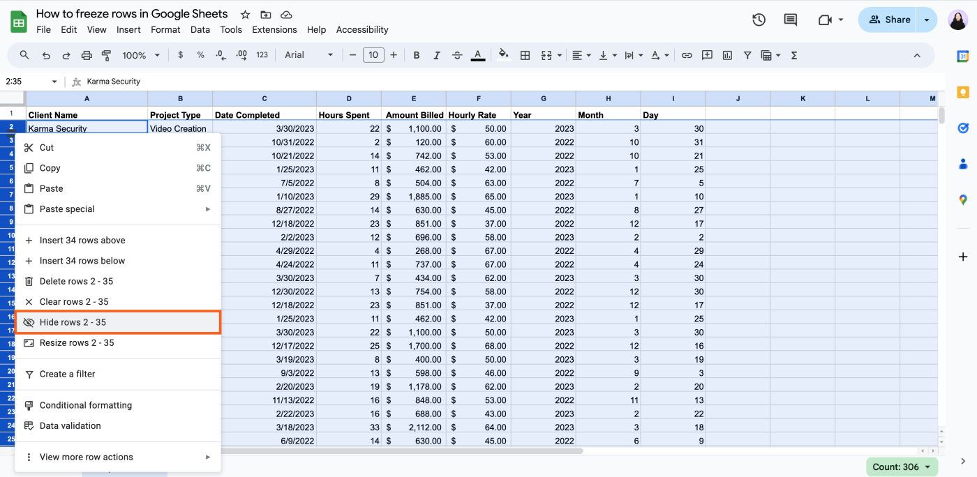

That's it. A pair of arrows will appear on the rows above and below your hidden selection to indicate there are hidden rows.

To unhide your selection of hidden rows, click the pair of arrows. Alternatively, select the rows above and below your hidden selection, and use your keyboard shortcut: command+shift+9 on Mac or Ctrl+Shift+9 on Windows.

Need to hide columns in Google Sheets instead? Select the columns you want to hide, right-click the selection, and click Hide columns [column letters]. The same pair of arrows will appear in the letter header on either side of your hidden selection. Click the arrows to unhide your columns.
If you want to prevent others from editing hidden columns or rows, check out how to lock cells in Google Sheets.
Automate Google Sheets
Scanning through spreadsheets is draining. And so is entering data manually. Use Zapier to connect Google Sheets with your go-to apps. This way, you can automate your most time-consuming spreadsheet-related tasks. For example, you can automatically add new lead data and form submissions to an existing spreadsheet. Learn more about how to automate Google Sheets, or get started with one of these workflow templates.
Collect new Typeform responses as rows on Google Sheets
Add Google Sheets rows for new Google Forms responses
Add new Facebook Lead Ads leads to rows on Google Sheets
Add new leads in LinkedIn Ads to Google Sheets rows
To get started with a Zap template—what we call our pre-made workflows—just click on the button. It only takes a few minutes to set up. You can read more about setting up Zaps here.
Related reading: