If numbers are involved, a spreadsheet's the tool for the job. But spreadsheets can also be used for so much more: storing contacts, compiling research, organizing outlines, and more.

With the right functions, you can use spreadsheets to quickly craft HTML, format links in Markdown, translate text, clean up copy, or perform any other bulk text editing task where you just might need a bit of automation help.

To take your spreadsheet-powered CRM further, or to make your own spreadsheet tools, here are the best text-focused features built into Google Sheets.

• Maintain an Editorial Calendar

• Build Detailed Outlines

• Import Data From Websites and Feeds

• Identify and Translate Text

• Format Text Automatically

• Combine Text from Cells

• Create Linked Text

• Display Images From a URL

• Write HTML Code

• Publish Your Spreadsheets

Maintain an Editorial Calendar

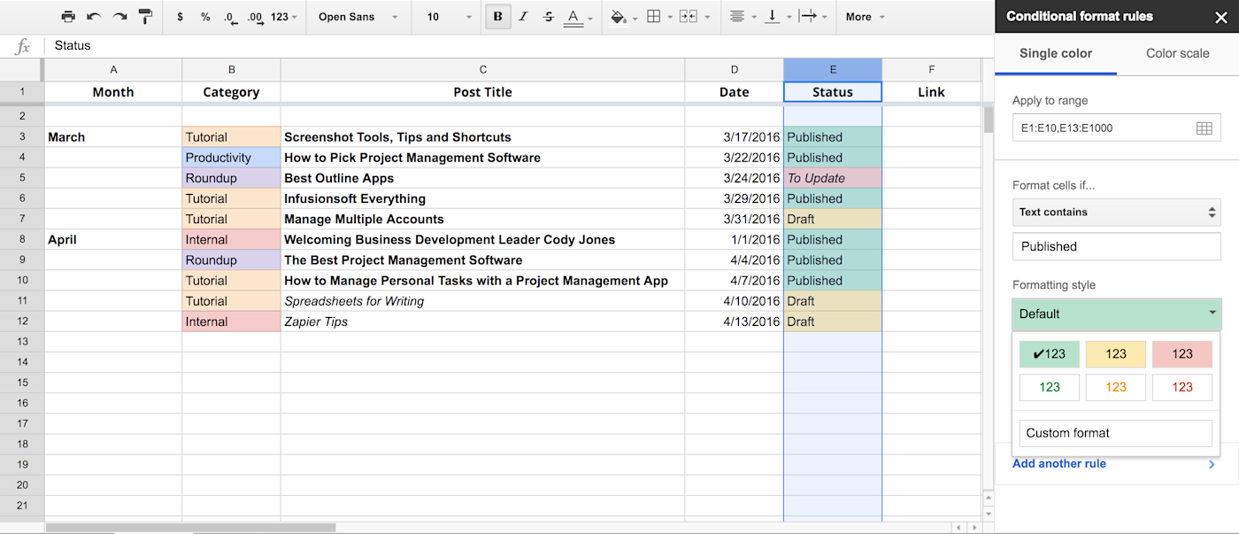
If there's one part of the writing process that seems obvious for a spreadsheet, it's the editorial calendar. With dates, word counts, topics, status, and budget to manage, a spreadsheet's unlimited columns and number-centric tools seem perfect.

And they are. Just take a bit of time to add columns for everything you want to track, something that will be a bit different for every blog, newsletter, or online publisher. You might not need to fill in each column for each piece: I've used a Month column that only gets filled in once to group articles by months, something that could work equally well to organize a blog's articles by day or a publisher's content by author.

Then, if you want to hide old items, you could select the rows under that month or another category, right-click and select Hide Rows. In Smartsheet, another spreadsheet app with more project-centric tools, you could indent the rows under that category—select the rows, then click the Indent button—and view or hide them with a click.

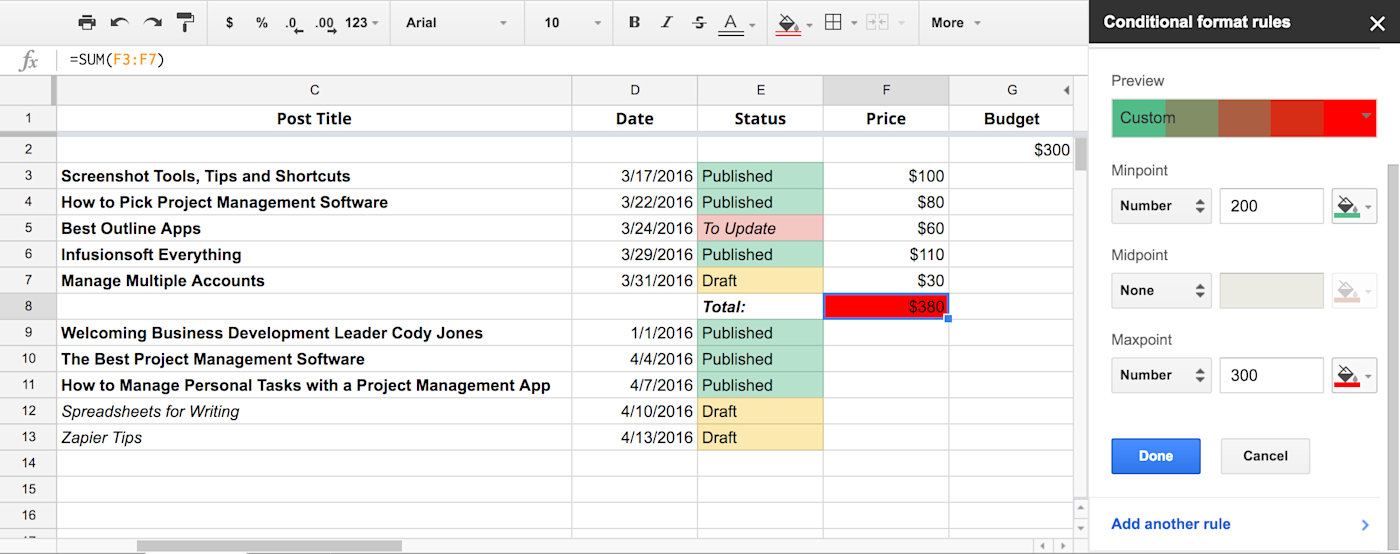
Have to keep this month's content within budget? Just add a column to track how much each article costs, along with perhaps another column to track this month's budget. You can then easily use =sum() and =Cell-Cell functions to see how close you are to your budget. Or, add conditional formatting from Format -> Conditional Formatting... to have Google Sheets change the color of your budget cell once you've gone over budget.

Track Published Items

Once you've planned the content you'll publish, it's time to turn those ideas into new posts. There's no reason to paste your titles into WordPress manually; app integration platform Zapier can watch for new rows—or newly updated rows, to watch for only article ideas that are Approved, say—and turn them into new draft posts in WordPress.

Another step on the Zap could then add the link to the draft post back to the spreadsheet. All you'll have to do is paste in your article content and hit Publish.

Or, you could link your spreadsheet to your productivity app. Say you use Trello to manage your article ideas and editorial process—the way the Zapier team manages our blog queue. Whenever a Trello card gets moved to the Published list, a Zapier automation could log that published article to your spreadsheet for a record of what's been published, including information such as word count and author.

If you use the spreadsheet to manage your blog's schedule and editorial workflow, a Zapier automation could create events in your calendar app or tasks in your to-do list app so you remember to edit and publish articles on time.

No matter what you want to track about your editorial process, a spreadsheet can be a valuable tool since it's so flexible. Then, just open another sheet, and it's time to start outlining the content you've planned.

Build Detailed Outlines

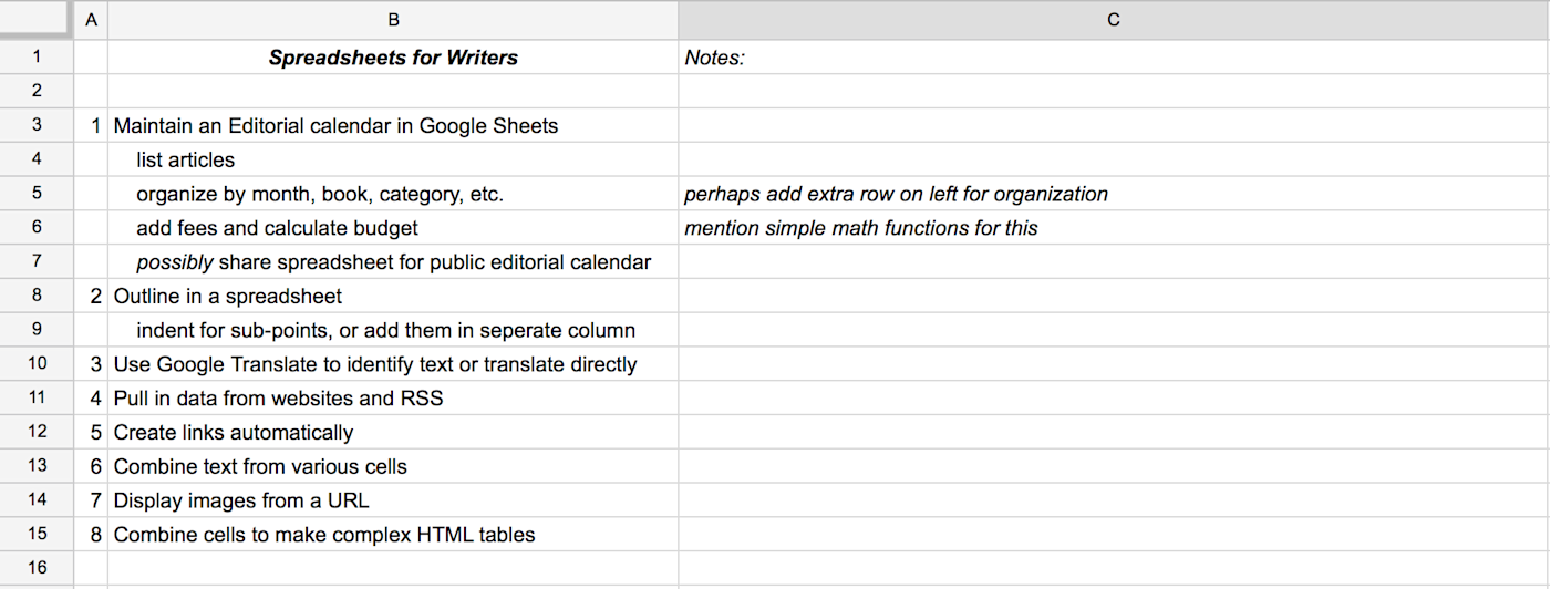
Once you've planned your content strategy, it's time to start turning those ideas into reality. First, outline your thoughts to make sure your articles and chapters flow in a logical order.

There are tons of outlining apps designed to organize ideas into detailed blueprints, and they're great. But so is your spreadsheet.

Just type each idea you want to cover in its own row—or if you've already typed it in a list, just paste the whole list and the spreadsheet app will add each to a new row automatically. Then, click and drag on the left-hand row number to rearrange ideas into the flow your piece needs.

With that done, it's time to flesh out the points with sub-points and notes. Perhaps add a new column for point numbers on the left, then add new rows for each sub-point with spaces or dashes to indent sub-points and make them stand out. Alternately, you could add sub-points in the next columns on the right, though that might be a bit harder to read.

You might not even need to type in your outline ideas. could bring in ideas from blog posts you read and notes you take. Perhaps favorite relevant tweets or add ideas to a project notebook, then have Zapier add those as new rows in your outline spreadsheet. All you'll have to do is organize the ideas once you're ready to write.

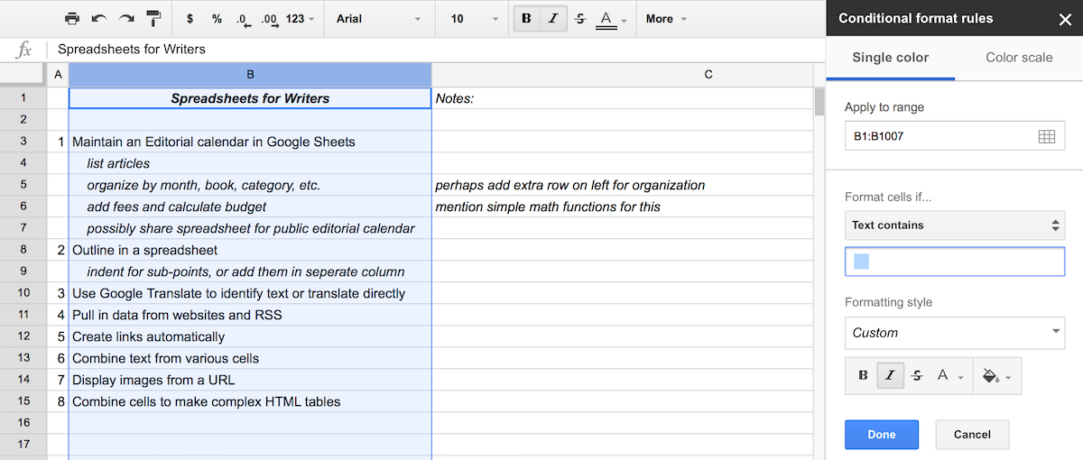
Want to make sub-points stand out even more, without adding formatting by hand every time? Just standardize the way you list sub-points—here, I've added four spaces before sub-points, but you could use a dash or other symbol instead. Then, add Conditional Formatting as above, only this time, apply it to your entire outline and have it watch for those spaces, dash, or other symbols. The formatting could add a new color, make the text italicized or bold, or add a background color.

For notes, those right-hand columns are a handy place to write extra text, list links that need to be mentioned, and gather anything else that your piece requires. You can then hide columns or sub-rows as needed to focus on your core outline—or, use conditional formatting again to make certain notes stand out from the others.

Import Data From Websites and Feeds

Want to pull articles and research into your spreadsheet? Google Sheets can import data from the web, automatically, right into your spreadsheet. You'll never have to open a new tab to research again.

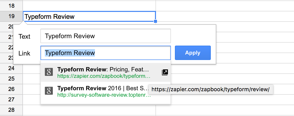
Start off by adding links to your ideas. Just select a cell in your spreadsheet, and press CMD+K or Ctrl+K to add a link. Google Sheets will search Google for that item, and return the first two search results for that phrase. You can then open the search result in a new tab, or just select the result to link that text to the site.

Or, you can import the most recent articles from an RSS feed right into your spreadsheet. Just enter your RSS feed in a cell, such as https://zapier.com/blog/feeds/latest/ for the Zapier blog. Then, in the next cell, enter this formula to import the titles of the five most recent articles (change A1 for the cell you entered the feed link in, and 5 for the number of results you want to import):

=importfeed(A1,"items title", false, 5)

Then, to get the links to those articles, enter this in the next column:

=importfeed(A1,"items URL", false, 5)

Now you've got the links and titles of posts. To turn them into linked text, enter this in another column, changing B2 for the cell with your article link and A2 for the cell with your article title.

=hyperlink(B2,A2)

With a bit of tweaking, that'll give you an RSS feed reader right inside Google Sheets, much like in the screenshot at the start of this section. You could use the IMPORT functions in Google Sheets to also import HTML, XML, or data from another spreadsheet. Jump back to the guide on scraping data with Google Sheets in Chapter 3 for more details on how to import specific data directly from links, and more.

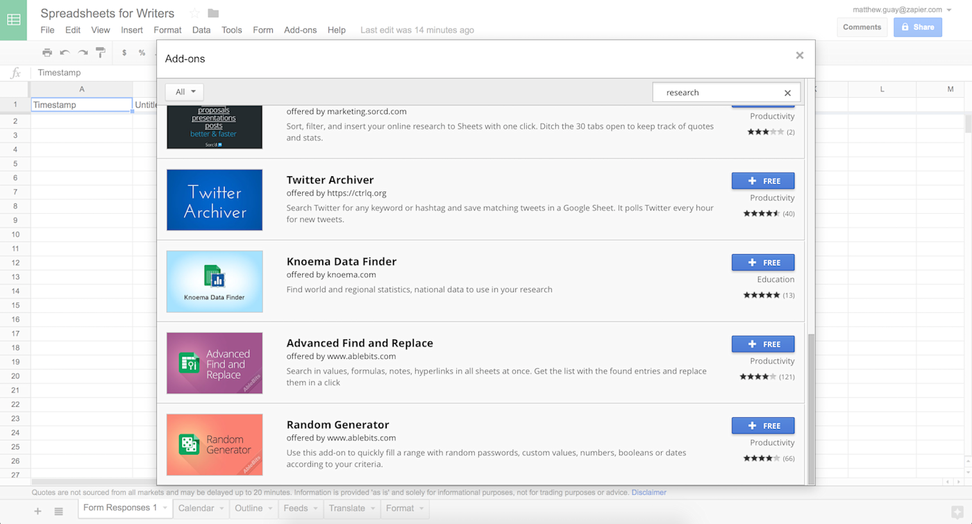
Or, you can install Google Sheets Add-ons to find extra info online and directly import it into your spreadsheet. We'll look at add-ons more in chapter 6, but for now, here are some of the best add-ons to search Twitter, Wikipedia, maps and other datasets:

• Wikipedia Tools: search Wikipedia, find synonyms for words, find categories, and import links and facts directly from Wikipedia.

• Knoema Data Finder: look up data and statistics about the world—including population and GDP—and insert them into your spreadsheet.

• Twitter Archiver: save Tweets to a spreadsheet, search Twitter, and research hashtags inside Google Sheets.

• Geocode by Awesome Table: turn addresses into latitude and longitude values, then can display those locations on a map in your spreadsheet.

• Advanced Find and Replace: search for text, formulas, and notes in specific parts of your spreadsheet—and replace them in only those sections if needed.

Gather Data Elsewhere and Import it to Your Spreadsheet

Want to gather new info over time, and have it added to your spreadsheet? Spreadsheet integrations could bring in ideas from the news, notes, and notifications.

As you're researching your article ideas, you could favorite relevant tweets or add ideas to a project notebook, then have Zapier add those as new rows in your outline spreadsheet. All you'll have to do is organize the ideas once you're ready to write.

Add Data Quickly With a Form

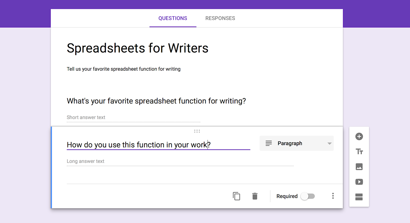
Another great way to gather research is with a form or survey. Google Sheets comes with a tool for that built in, which we looked at in chapter 2: Google Forms. Just click Tools -> Create a Form, and a new tab will open with a form editor where you can add questions to a quick form or survey.

Save and share the form, and Google Sheets will automatically save the responses back to a new sheet in your original spreadsheet. Then, you can incorporate those responses into your research, right alongside everything else you've pulled into your spreadsheet.

Be sure to jump back to chapter 2 for an in-depth guide to all of Google Forms' features if you haven't read it already.

Identify and Translate Text

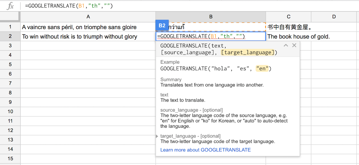
Come across some text you can't read in your research, or want to reference a quote in another language and include a rough translation? Google Translate is built into Google Sheets, and can identify or translate languages for you on the fly.

Identifying languages is simple. Just enter the text you can't read in a cell, then use the =DETECTLANGUAGE(A1) function, replacing A1 with your text cell. Google Translate will then tell you the two letter code of that language: en for English, th for Thai, fr for french, and so on.

Then, to translate text, just enter the following formula:

=GOOGLETRANSLATE(A1,"auto","en")

That will translate the text in cell A1 into English, after auto-detecting the language. You can replace auto with the two-letter code for the language if you already know what language the text is in, or swap en for any other language for other translations.

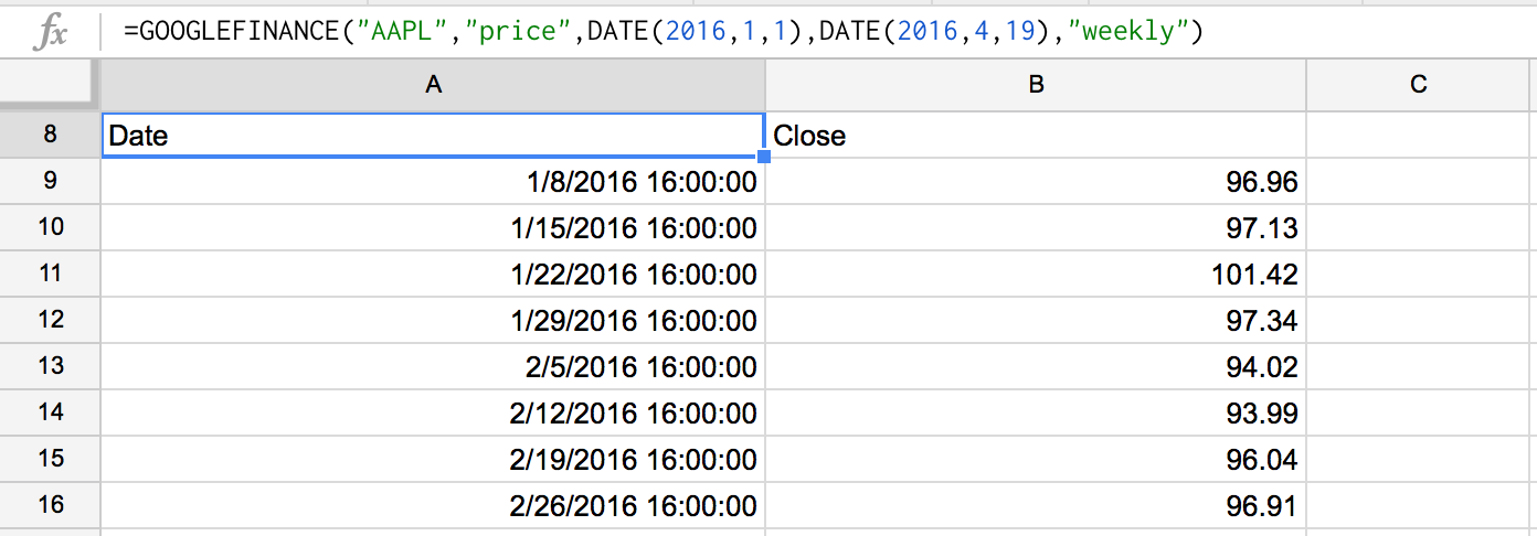
Need to translate cryptic financial terms instead of languages? Google Finance's integration into Sheets is just what you need. Just enter =GOOGLEFINANCE() with your stock ticker, the item you wish to track, start and end date, and daily or weekly for how you want the data summarized, and you'll get a table of stock results automatically. That might be helpful for your next article on the stock market.

Format Text Automatically

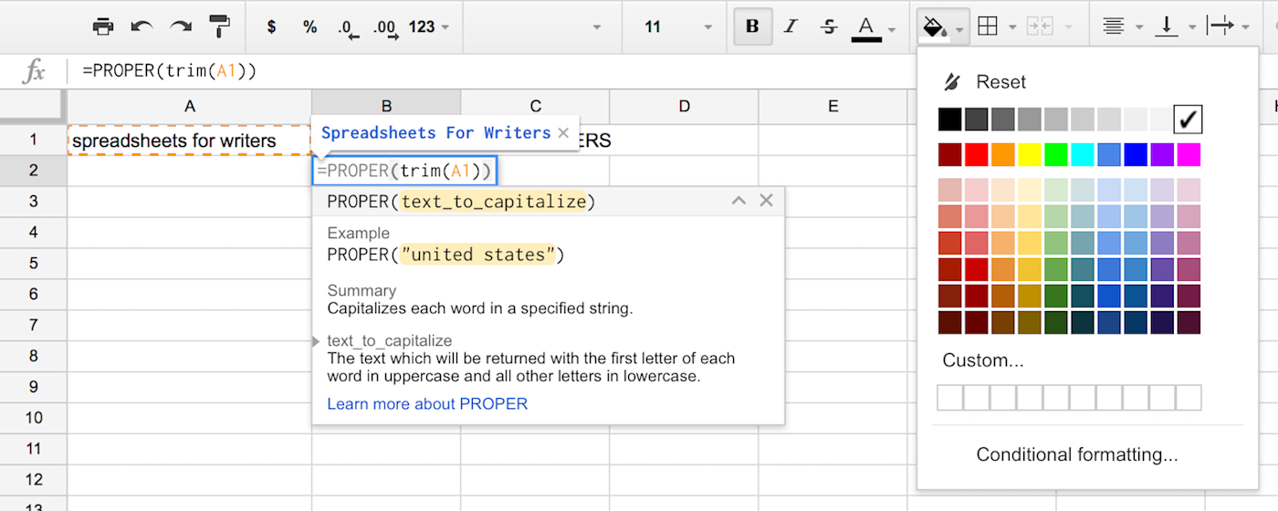
Now that you've got an outline, notes, and research in your spreadsheet, it's time to get things cleaned up. You've likely used the formatting options in spreadsheets before—if not, they work the same as you'd expect in most other office applications. Select the font, size, and weight you want for text, pick text and background colors, center or left/right align text, and so on. Or, use the Conditional Formatting tool we've already looked at to change colors and font style based on what's in each cell in a spreadsheet.

One spreadsheet-specific formatting option to try is the Borders option. That lets you choose which—if any—borders to show around cells, as well as what color and thickness the lines should be. Turn off all the borders, and your spreadsheet will look like a plain document.

Then, Google Sheets can help automatically clean up your text to make it look the way it should. Here are some of the best Text functions you should use (and replace A1 with text you want to clean up, as usual):

• Clean(A1) to remove non-printable ASCII characters, useful for making imported HTML or XML look better.

• Left(A1,5) or Right(A1,5) to return the first or last 5 (or any number you want) characters from a string, respectively.

• Trim(A1) to remove any leading or trailing spaces.

• Upper(A1) to make all of the text uppercase.

• Lower(A1) to make all of the text lowercase.

• Proper(A1) to capitalize the first letter of each word.

• Substitute(A1,"text_to_search_for","text_to_replace_with") to replace something in a string with something else (say, to replace one word or remove all spaces).

You can also combine text functions. For example, in the image above, =Proper(Trim(A1)) both removes the spaces from the end of the string and capitalizes the first letter of each word.

Combine Text from Cells

There's another super handy Text function for combining text from multiple cells in a spreadsheet: Concatenate. All it does is combine the text you enter or select form cells together into one cell. If you want to add spaces, you'll need to add them manually: concatenate just combines the exact text you give it.

Here's how it's handy: Say, for instance, you've written an article and included anchor tags so readers can jump to a specific section of the article from your index—perhaps using a lower case version of the app's name, without spaces, for the anchor tags. You want to make an index for that article, which means you need a list of links with each of those anchor tags and your article's URL.

Instead of writing each anchor in lowercase by hand, just paste your list of Anchors into a spreadsheet. Then, add the following formula, substituting your link for URL and your anchor's cell in the spreadsheet for A1:

=concatenate("URL",A1)

Or, if you need to make the anchor text lowercase and remove spaces, this function would do the trick:

=concatenate("URL",lower(substitute(A1," ","")))

Create Linked Text

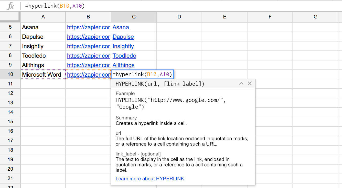
Once you've got the links, you might want to link the original anchor names with their new anchor links. The Hyperlink function can do that for you. Just enter the following, with your link and text instead of B1 and A1, respectively:

=hyperlink(B1,A1)

That will make a new column with the original text linked to your new links—and it'd work equally well with any list of plain text and links.

If you write in Markdown, you could instead use concatenate to add brackets and parenthesis with this function, where again A1 is your plain text and B1 is your link:

=concatenate("[",A1,"](",B1,")")

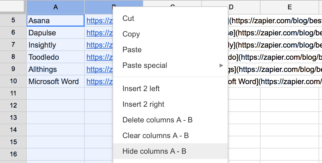
Want to only show the linked text, instead of three columns with plain text, plain link, and linked text? Just select the text and link columns, right-click on the top header, and select Hide Columns. The text will still be in your spreadsheet, and will still work in functions, but it'll be out of sight to keep your spreadsheet clean.

Or, want to save only the new links, without the functions and original text? Just copy the original hyperlinks you made, paste them in a new column, then click the paste icon that shows up and select Paste values only.

Display Images From a URL

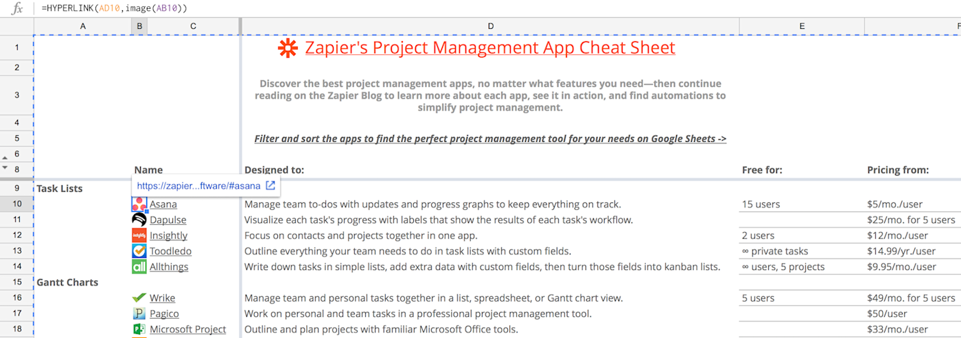
Spreadsheets aren't just for numbers, and they're not just for text either. They're also great places to organize images.

Most spreadsheet apps let you drag-and-drop images into your spreadsheet, perhaps to add a company logo to your financial statements. But Google Sheets also lets you import images directly from a link with its image function.

We recently used this in the Zapier team to build a project management apps comparison tool. I added each icon to Zapier's site, and listed them in the spreadsheet—right after the anchor links I'd made with the trick in the previous step. Then, I added both a hyperlink and image function, as below, to both import the image and have it linked to the correct section of our article:

=hyperlink(A1,image(B1))

The image function also lets you set a mode, height, and width. The mode could let the image automatically fit the height or width of the cell, or you could just set the size manually.

There's only one problem with these online images: they only work in Google Sheets. They're perfect if you want to view the spreadsheet online or export it as a PDF, but if you save it in Excel format, the images won't be saved with it.

Alternately, if you want a full-sized image, just select Insert -> Image then upload a photo or search for one in Google Images. You can then resize and position the image anywhere on your spreadsheet, as it's not tied to any specific cell. The image function is handy for pulling in a number of images at once and showing them in a table; the Insert Image tool is better for adding full-sized images for a nicer looking report.

Create HTML Tables For Your Blog Posts

It's time to bring everything you've learned together. Let's turn your outline or list of ideas into an HTML table that you can add to your finished blog post—complete with anchor links to the correct sections of your article.

Just set up your spreadsheet with each thing you want to include in the table (like text, links, and images), then kick off a concatenate function. For example, in our Project Management app roundup, we include a table with each app's name, icon, description, and price. Here's the table we started with—column D was made using the Format tools mentioned above:

Or, perhaps you'd rather publish your spreadsheet itself instead of turning it into a table. There's a number of ways you can do that in Google Sheets:

• Export: Click File -> Download as to download your spreadsheet in Excel, CSV, web page, or PDF formats. The PDF option is a great way to share your writing, outline, and research with others, while the spreadsheet options are best for backing up data to use in other spreadsheet tools.

• Print: For a bit more formatting options—though no way to export links—click the printer icon. You can then print the sheet on paper, or save it as a formatted PDF to Google Drive.

• Publish: Click File -> Publish to the Web to get a public link to your spreadsheet to share a plain HTML page of your spreadsheet with others. Or, click the Embed tab, copy the code it includes and paste it into your blog to embed a copy of the spreadsheet in your post instead of making an HTML table.

Each of those options only let you share a plain, static copy of your spreadsheet. If you want readers to be able to sort and filter through your data, though, you'll want to actually share the real spreadsheet.

For that, click the Share icon in the top right corner, and select Anyone with the link can view from the sharing options. Then, share the link, and anyone can view the spreadsheet, and search through the data without changing the original layout.

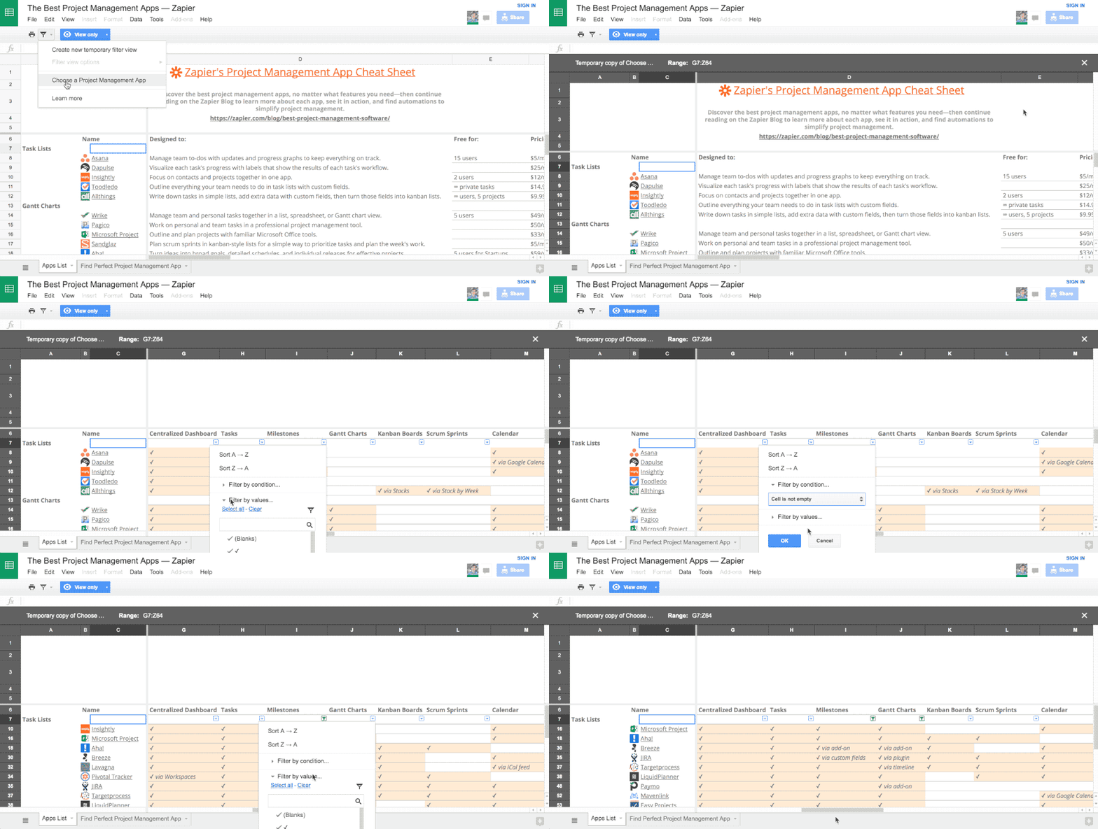
For a better way to help people find the items they need, add a Filtered View from Data -> Filter View. There, you can set which part of the spreadsheet should be interactive. Readers can then click on a column, filter it by name or text, and see only the results they want. You could even make filter views with preset filters that only show specific data, as an easy way to sort through massive datasets.

Spreadsheets still aren't exactly word processors, and you'll still want a writing app for most of your writing work. But for research, outlining, tables, and much more, a spreadsheet is a handy sidekick that can help you do more, in far less time.