When you're staring at endless rows of data in a spreadsheet, it can be hard to make sense of what it all means. And if you're scrambling to put together a presentation on the key takeaways from that spreadsheet—forget about it.
That's why I use conditional formatting. It lets you format rows and columns, which not only makes large data sets less of an eyesore but also makes your spreadsheet easier to digest.
I've covered how to do this in Google Sheets. But if you're a Microsoft user, here's how to use conditional formatting in Excel.
If you're looking for a quick refresher, here's the short version of how to use conditional formatting in Excel. (Scroll down to learn more specifics and practice with a demo spreadsheet.)
Select a range.
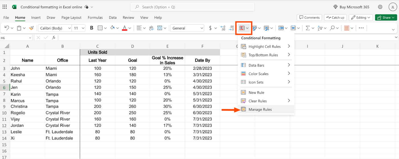
In the Home tab of your ribbon, click Conditional Formatting. Then select Manage Rules.
In the Conditional Formatting panel that appears, click the New Rule icon, which looks like a plus sign (
+).Select the rule type (and, if needed, customize the condition).
Select the formatting style.
Click Done.
What is conditional formatting?
Excel's conditional formatting feature lets you dynamically format a cell's background and text style based on custom rules that you set. A rule in Excel operates as an if/then statement.
If you've used Zapier before, the rules of conditional formatting might sound familiar. It works a lot like a Zap (what we call our automated workflows): if the trigger event happens, then the action will follow.
Using our demo sheet, let's say we want to highlight any cells displaying less than 100 units sold in the last year. To do this, we would use the conditional formatting rule shown below, which tells Excel, "If any cells between cells C3 and C14 contain a value of less than 100, then change that cell's background color to light yellow."

Before we continue, it's important to understand the three key components that make up every conditional formatting rule.
Range: A range can be anything from a single cell to multiple cells across different rows and columns. The range indicates which cell (or cells) the rule applies to. In the example above, the range is C3 to C14.
Condition: This is the "if" part of the if/then rule. You can choose from more than a dozen options, including greater than, less than, between, and so on.
Formatting: This is the "then" part of the if/then rule. It refers to the formatting that should apply to any given cell if the conditions are met. In the example above, the style is "background color to light yellow."
How to use conditional formatting in Excel
Conditional formatting helps make your data stand out. Here's how to create and modify conditional formatting rules in Excel.
For this tutorial, I'll show you how to create a rule to find out which employees sold more than 140 units last year.
To follow along, use our demo sheet. You can save a copy to OneDrive and follow along online. Or you can download a copy to your computer to follow along in the desktop app. (Note: I use the web version of Microsoft Excel, but the steps are pretty much the same in the desktop app.)
1. Select a range
There are two ways to select your desired range. If you're not working with a lot of data, the fastest way to do it is to highlight the range directly in the spreadsheet. If you're creating a rule for a large data set, you're better off inputting the range manually. Here's how.
In the Home tab of your ribbon, click Conditional Formatting. Then select Manage Rules.
In the Conditional Formatting panel that appears, click the New Rule icon, which looks like a plus sign (
+).In the Apply to range field, input your range.
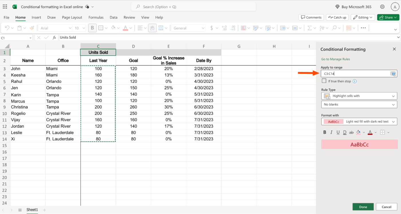
Click Done.


2. Create the rule
Once you've selected your range, create your rule (your if/then statement). If your Conditional Formatting panel is open, you can create your condition in the Rule Type section.
If not, click Conditional Formatting in the Home tab of your ribbon. The most common rules are grouped under two categories: Highlight Cell Rules and Top/Bottom Rules. (To learn more about how to use each formatting rule, jump to the bottom of this article.)

For some reason, Excel doesn't group the different rule options the same way in the Conditional Formatting panel as it does in the Conditional Formatting menu from the Home tab—but you can choose from all the same rules in either section. For this section of the tutorial, we'll create our rule from the Conditional Formatting panel.
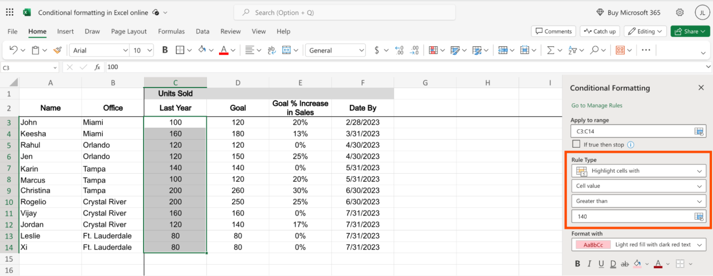
As a reminder, we want to create a rule to highlight cells displaying more than 140 units sold last year. To do this, we need to highlight cells using the Greater than rule.
In the Rule Type section, leave the default selection (Highlight cells with) as is.
Click the second field, and select Cell value. This will automatically populate two new fields.
In the third field, leave the default selection (Greater than).
In the fourth field, enter the Greater than value. In this case, enter 140.

Note: If you add more than one conditional formatting rule to a given range, Excel will run through each rule in the order they were created. But once a rule is met by any given cell, subsequent rules won't override it.
3. Select a formatting style
By default, Excel will format any cells that meet your rule with a light red fill and change the text to dark red. But you can change the formatting to anything you like.
In the Format with section, you can click the down caret (⋁) to choose from five other preset formatting styles. Or you can create a custom style using the formatting tools.
Since we want to highlight a positive outcome, let's change the fill color to light green and set the text color to black. Then click Done.

Excel will highlight any cells that meet your rule with a light green fill and black text. Now we can easily tell that Keesha, Christina, Rogelio, and Vijay all sold over 140 units last year.

To delete a conditional formatting rule, hover over the rule in the Conditional Formatting panel. Then click the Delete icon, which looks like a garbage can.

Let's say you've created multiple rules, and you want to delete them all in one fell swoop. Beside Manage Rules, click the Delete all rules icon, which looks like a garbage can.
Types of conditional formatting rules and styles
Now that you know how to create conditional formatting rules, let's explore all the conditional formatting rules in Excel.
Highlight Cell Rules
Common Highlight Cell Rules like Greater than, Less than, Equal to, and Between are self-explanatory, so let's review the last three available options: Text that contains, A date occurring, and Duplicate values.
Text that contains rule
This rule will highlight cells that contain particular text. This can be useful if, say, you want to see how many times a name comes up. In our demo sheet, we can use this rule to visually separate employees from Tampa.

A date occurring rule
This rule will highlight cells that contain a date from today, yesterday, last week, last month, and so on. It's a dynamic rule, which means that the cells that meet the condition will change relative to the current date.
In the example below, I created a rule to highlight cells with a date occurring in the last month. Since I created the rule at the end of August 2023, Excel highlighted cells F11 to F14, which contain the date 07/31/2023. If I created the same rule in, say, April 2023, only cell F4 (03/31/2023) would be highlighted.

Duplicate values rule
This rule is used to find repeat values within the given range.
If you want to find unique values (data that's not duplicated), this is just as easy to do. Create a new rule in the Conditional Formatting panel. In the Rule Type section, click the second field, and select Unique values.
In the example below, I used the Unique values rule to highlight any unique sales goals between cells D3 and D14.

Top/Bottom Rules
Top/Bottom Rules help you quickly highlight the best and the worst performers from a selected range—no complicated formulas required.
There are no customization options for the Above Average and Below Average rules, meaning you can't specify the average, but rules like the top and bottom 10 items and top and bottom 10% can be modified to meet your needs.
For example, you can change the Top 10 Items rule to highlight the top one, five, or even 100 items. In our demo sheet, we can use this rule to highlight your highest-performing employees based on which three sold the most units last year.

Conditional formatting styles
There are three other Conditional Formatting options, which are used to help visualize your data: Data bars, Color scales, and Icon sets.
Data bars
Data bars allow you to add dynamic bar graphs in the background of each cell. The bars are filled relative to other cells within the given range. For example, in the demo sheet, I applied a data bar to units sold last year (cells C3 to C14). The most number of units sold in this range is 200, so any cells containing this value also show a bar graph spanning the entire cell. Meanwhile, the least number of units sold in this range is 80, so any cells containing this value show a bar graph that spans less than half the width of the cell.

Color scales
Color Scales lets you take a backseat on choosing the formatting style. Once you specify the rule range and type, Color Scales automatically applies a color-based hierarchy system, so you don't have to.
There are multiple scale options available. The most commonly used one is the Green - Yellow - Red Color Scale. When applied, as shown in the example below, it will add a green background to cells containing the highest values and a red background for the lowest cell values. Cells containing values in between will be split using shades of orange and yellow.

Icon sets
Icon sets is a dynamic feature that functions similarly to Color Scales. You can pick from different icons, like arrows, shapes, and indicators, which are then added to each cell based on the cell's numeric value. The icons will also automatically update if the cell values are changed.
In the example below, I used the 3 Triangles icon set for cells C3 to C14. Cells with the highest values have an upwards-facing green arrow; cells with the lowest values have a downwards-facing red arrow; and cells with values in between have a light-orange bar.

Automate Microsoft Excel
Now that you know how to make your spreadsheet easier to digest, it's time to streamline your Excel-related tasks. By pairing Excel with Zapier, you can automate common processes like logging form submissions and notifying your team about updates to a spreadsheet.
Learn more about how to automate Excel, or get started with one of these workflows.
Add new Typeform entries as rows on an Excel spreadsheet
Related reading:
This article was originally published in July 2019 by Khamosh Pathak. The most recent update was in August 2023.