Truthfully, I can't be trusted with anything nice—and this extends to beautifully formatted, formula-filled Google Sheets spreadsheets. I get all click-happy, and the next thing I know, I'm staring at empty cells where there were once data-filled cells.
Sure, I could hit Undo, but that's helpful only if I know what errors I need to undo. Or the person sharing their spreadsheet with me could limit my permissions to view or comment only. But that's not practical if we need to collaborate on the file.
Google rightfully predicted there were more click-happy humans like me, which is why they added the ability for users to protect certain cell ranges and sheets from being tampered with.
Here's how to lock cells and sheets in Google Sheets.
Table of contents:
How to lock cells in Google Sheets
Open a Google Sheets spreadsheet.
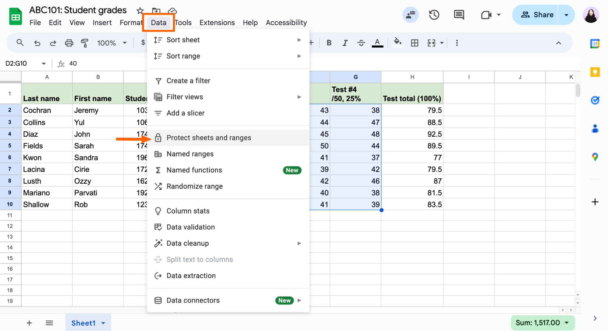
Highlight the cell or cell range you want to protect.
Click Data > Protect sheets and ranges. Alternatively, right-click your selection, and then click View more cell actions > Protect cell range.
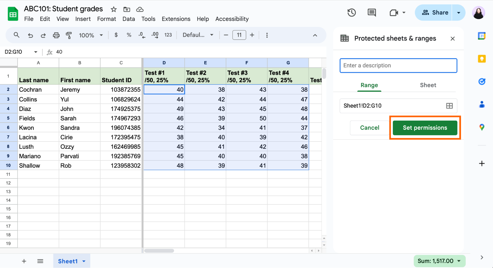
In the Protected sheets & ranges panel that appears, click Set permissions.
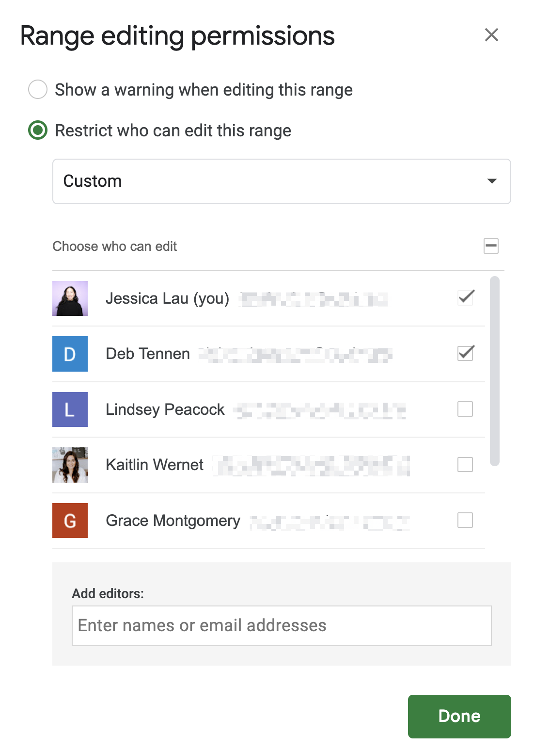
Modify the Range editing permissions in one of the following ways:
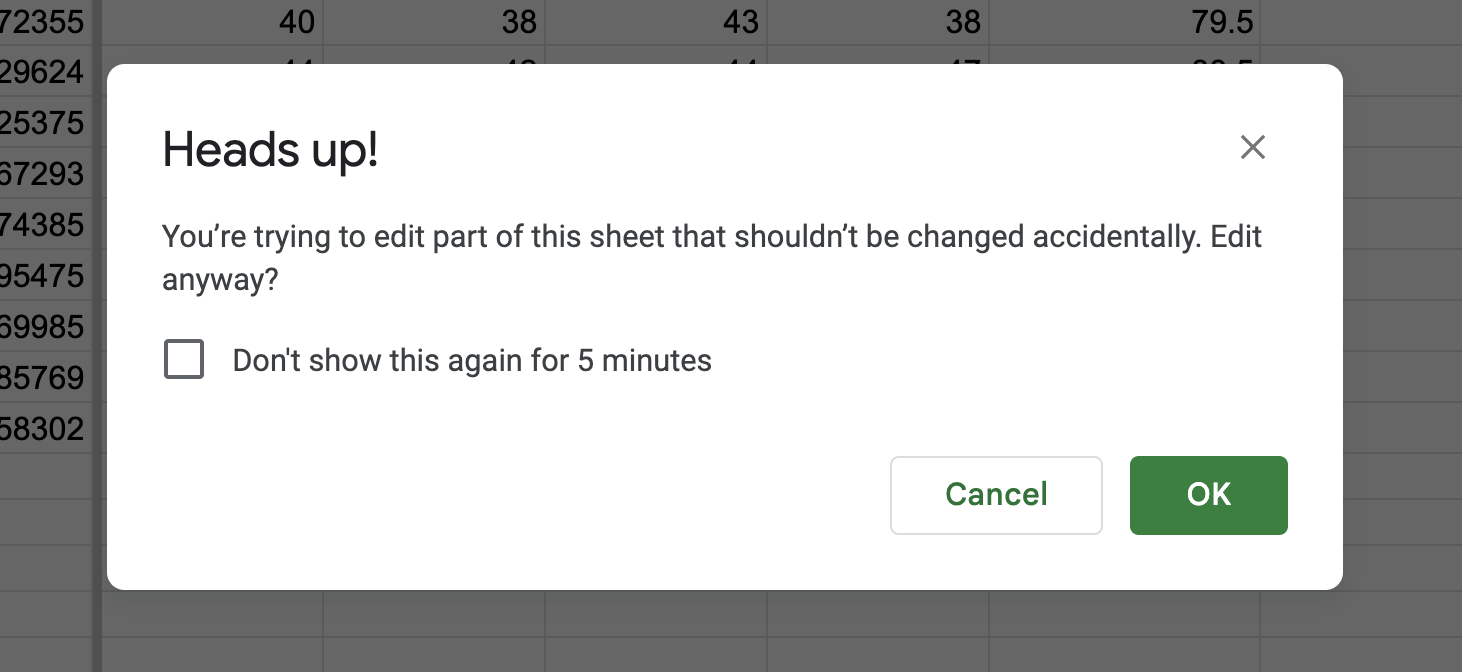
Show a warning when editing this range. Other users can still edit the protected range, but they'll get a warning first. This is a good option for dealing with click-happy collaborators.
Restrict who can edit this range. You can limit this to Only you. Or you can apply custom settings, giving specific people permission to edit the range.
Optionally, in the Protected sheets & ranges panel, enter a description for the locked cells. This is especially practical if you're managing multiple locked sheets and cell ranges.
Click Done.
Now, when someone who doesn't have permission to edit a cell range tries to modify it, they'll get a popup notifying them that the cell is protected and to contact the spreadsheet owner to remove the protection, if needed.

How to lock an entire worksheet in Google Sheets
Let's say you have multiple worksheets in your spreadsheet and you want to lock specific worksheets. Here's the easiest way to do it.
Click Data > Protect sheets and ranges. Or right-click any cell, and then click View more cell actions > Protect cell range.
In the Protected sheets & ranges panel that appears, click Sheet.
Select the sheet you want to lock.
Optionally, check Except certain cells to make certain cells within the locked sheet editable.
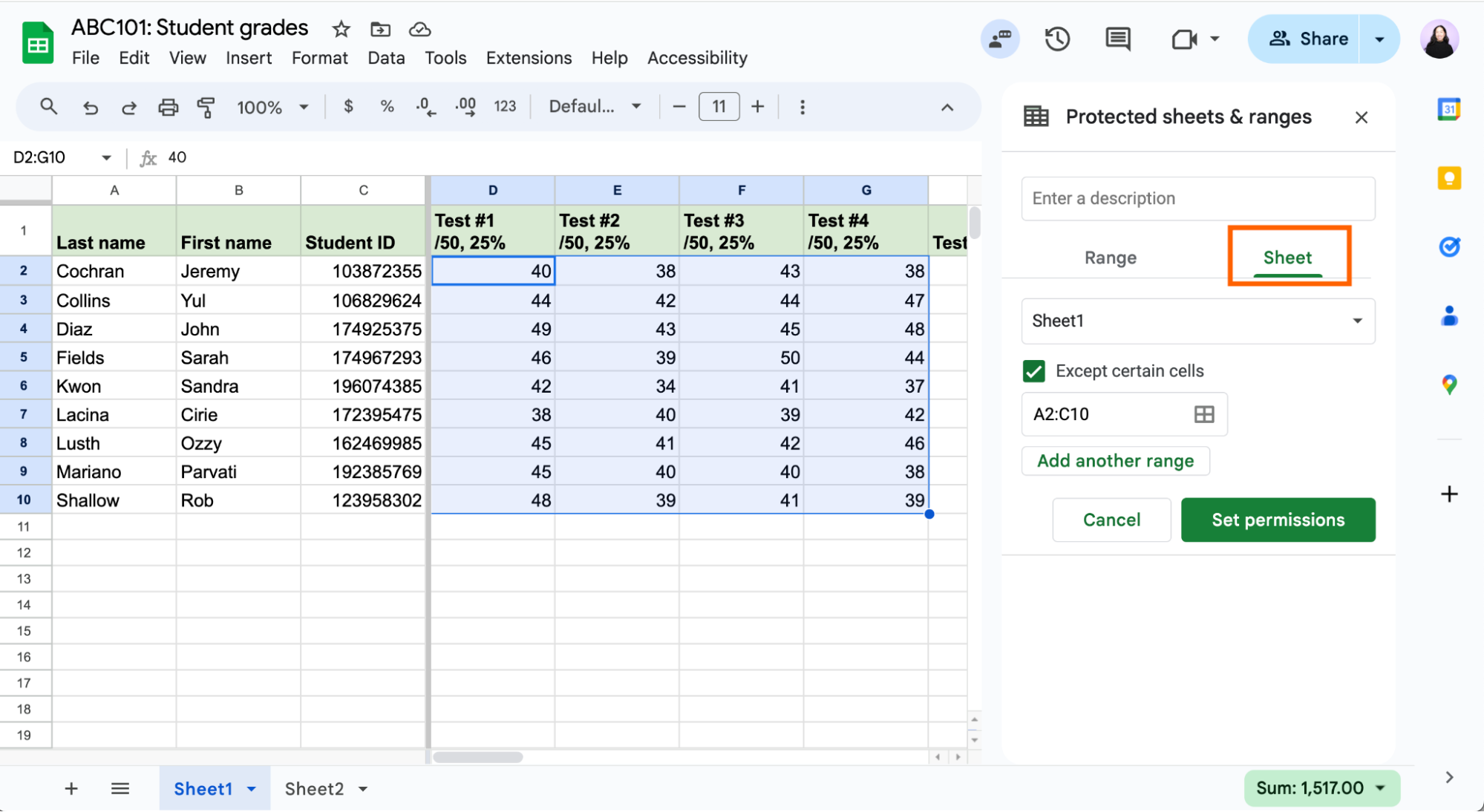
Click Set permissions.
How to edit locked cell settings in Google Sheets
How to edit the cell range of locked cells in Google Sheets
Click Data > Protect sheets and ranges. Or right-click any cell, and then click View more cell actions > Protect cell range.
Click the locked cell range you want to edit.
To modify the range of locked cells, manually enter a new range in the Select range field. Or click the Select data range icon, which looks like a grid, highlight the new cell range directly in your worksheet, and then click OK.
Click Done.
How to change editor permissions of locked cells in Google Sheets
Click Data > Protect sheets and ranges. Or right-click any cell, and then click View more cell actions > Protect cell range.
Click the protected sheet or cell range you want to edit.
Click Change permissions.

Update the Range editing permissions.
Click Done.
How to unlock cells in Google Sheets
Click Data > Protect sheets and ranges. Or right-click any cell, and then click View more cell actions > Protect cell range.
Click the protected sheet or cell range you want to edit.
Click the Delete range or sheet protection icon, which looks like a garbage can.

Automate Google Sheets
There are countless ways to accidentally mess up a spreadsheet—the process of entering data doesn't have to be one of those ways. Use Zapier to connect Google Sheets with your go-to apps. This way, you can automatically do things like add new lead data and form submissions to an existing spreadsheet. Learn more about how to automate Google Sheets, or get started with one of these workflow templates.
More details
More details
More details
To get started with a Zap template—what we call our pre-made workflows—just click on the button. It only takes a few minutes to set up. You can read more about setting up Zaps here.
Related reading: