How to add a checkbox in Google Sheets

A checked box in Google Sheets has no business sparking as much joy as it does. But here we are.

Here, I'll show you how to add a checkbox in Google Sheets—plus, a few advanced tips to make your checkboxes do more than just check a box.

Table of contents: 

• How to add a checkbox in Google Sheets

• How to add a checkbox in Google Sheets: Advanced tips 

How to add a checkbox in Google Sheets

There are two ways to add a checkbox in Google Sheets. Here's the quickest method. 

1. Open the Google Sheet that you want to edit. 

2. Highlight the cell range where you want to insert checkboxes.

3. Click Insert, and then select Checkbox. 

That's it. Now you can feel productive—even if you're just checking off tasks like "open spreadsheet" and "add checkbox."

How to add a checkbox in Google Sheets: Advanced tips

Adding checkboxes on their own won't win you any spreadsheet street cred. But combine them with conditional formatting, and suddenly your coworkers are endorsing your spreadsheet skills on LinkedIn.

Here's how you can use conditional formatting to get your checkbox to do even more in Google Sheets. 

1. Change the checkbox value 

By default, Google Sheets sets the value of checked boxes as TRUE and unchecked ones as FALSE. But if you're using checkboxes to trigger conditional formulas, automation, or filters, it's more practical to customize your values to something more intuitive—like "Approved/Pending" or "Complete/Not started." It'll also make your data easier to work with if you export it to another app or share it with others. 

Here's how to change the checkbox value in Google Sheets.

1. Click Data, and then select Data validation. 

2. In the Data validation rules side panel, click Checkbox. 

   

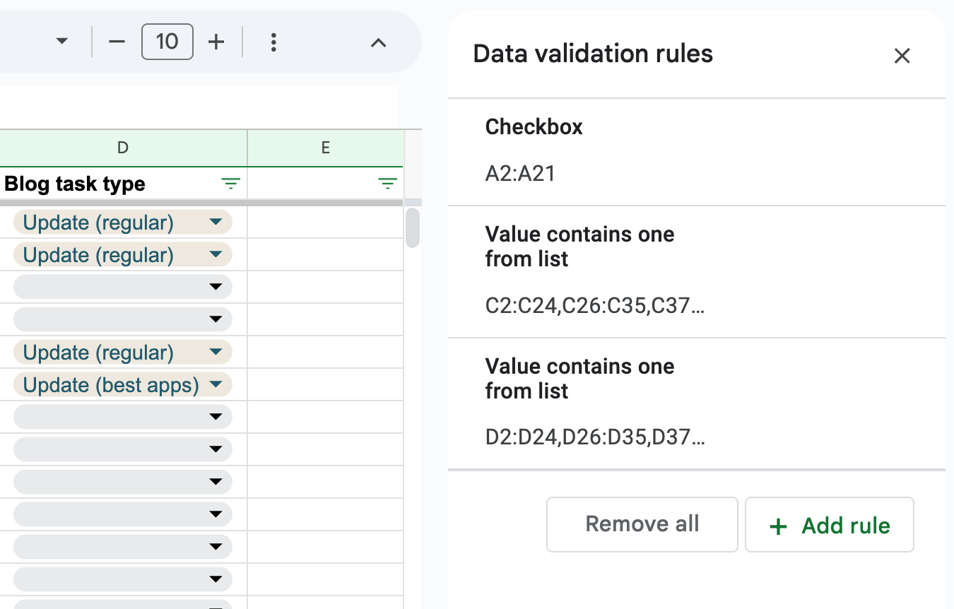
3. Click the Use custom cell values checkbox. 

4. Enter your custom values for Checked and Unchecked. 

   

5. Click Done. 

Now no one has to guess why there's a TRUE/FALSE value for "Was Leroy the office dog fed his max quota for treats today?" 

2. Strike through your task list 

If you use Google Sheets as your to-do list, you can automatically cross out entire rows as you check off your tasks. Seeing a line run across your entire row provides infinitely more satisfaction than seeing only a tiny checkmark go through one solitary box. 

1. Highlight the cell range that you want to apply conditional formatting to (include your column with checkboxes).  

2. Click Format, and then select Conditional formatting. 

3. In the Conditional format rules side panel, click Add another rule. 

4. Click the Format cells if dropdown, and select Custom formula is. 

5. Enter this formula: =$[checkbox column][row number]="[checkbox value]". In this example, the formula is =$A2="YES". Note: The dollar sign ($) locks the reference to the given column while allowing the row number to change dynamically down the column. 

6. Select how you want your text to be formatted if it meets the criteria. In this example, I set it to strike through text and fill the row with light gray.

   

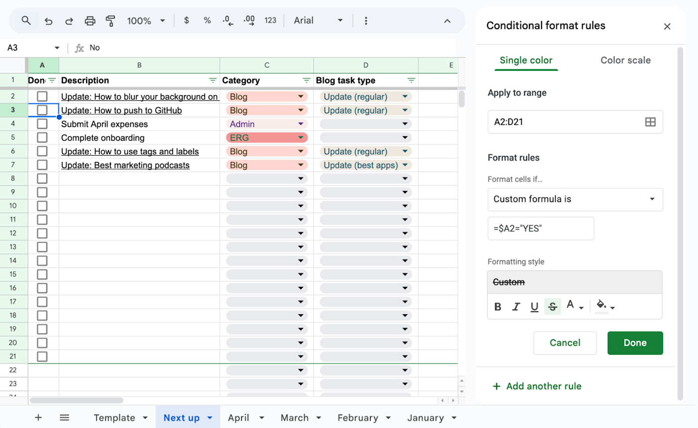
7. Click Done.

   

See? Way more satisfying. 

Automate Google Sheets 

Checkboxes—with the help of a few different formulas—can do quite a bit inside Google Sheets. But there's no way your tech stack consists of just Google Sheets. 

When you use Zapier's Google Sheets integration, you can connect it with thousands of other apps. This way, you can automatically do things like get Slack notifications whenever there's an update to your sheet or add data to your sheet from other sources, including your CRM, email, or anywhere else you can think of. Learn more about how to automate Google Sheets, or get started with one of these pre-made templates.

Related reading: 

• How to create a calendar in Google Sheets

• The best Google Sheets add-ons to boost your productivity

• Google Sheets shortcuts to help you enter, organize, and interpret your data